Week 9: Multilevel Modeling and Time-Series Forecasting

Why This Topic Matters

Behavioral data are almost always structured. Responses are nested within sessions, sessions are nested within participants, and participants are nested within clinics or classrooms. When you collect data from multiple individuals across multiple time points, you have a hierarchical dataset whether you intended to or not. Once made aware, the question is how to deal with it well.

Ignoring nesting is dealing with it poorly. When observations within a group (e.g., repeated measures from the same participant) are more similar to each other than observations from different groups, they are not independent. Standard regression and ANOVA assume independence. Violating this assumption inflates Type I error rates, sometimes dramatically. This can lead you to think you have found an effect when you have found noise that was correlated within people.

Multilevel models, also called hierarchical linear models or mixed-effects models, handle nesting explicitly. They decompose variance into within-group and between-group components. They allow each participant to have their own intercept, their own slope, or both, while still estimating overall effects. They pool information across groups, so that participants with sparse data are informed by participants with rich data.

But nesting is not the only structure in behavioral data. Behavioral observations are also sequential. Today's response rate is not independent of yesterday's. A participant who had a high-rate session on Monday is likely to have a high-rate session on Tuesday. This temporal dependence is autocorrelation, and ignoring it can lead to poor predictions and misleading inferences.

Time-series models handle temporal dependence directly. Autoregressive models capture the idea that the current value of a series depends on its recent past. ARIMA models extend this to handle trends and other nonstationarities. Time-series tools are essential for anyone working with repeated behavioral observations over time (i.e., nearly everyone in behavior science).

This week brings these two families of models together. Multilevel models handle the between-person structure. Time-series models handle the within-person temporal structure. Together, they provide a principled framework to analyze the kinds of data that behavior scientists collect.

Core Concepts

Why Nesting Matters

Consider a study in which you measure response rate across 10 sessions for each of 5 participants. You have 50 data points, but you do not have 50 independent data points. The 10 observations from Participant 1 share everything that makes Participant 1 unique such as their learning history, their sensitivity to reinforcement, and their baseline activity level. Those observations are correlated with each other, and that correlation means they carry less information than 50 truly independent observations.

If you ignore this and run an ordinary regression treating all 50 observations as independent, your standard errors will be too small. Confidence intervals will be too narrow. p-values will be too liberal. You will claim effects are significant when they are not. The severity of this problem depends on how similar observations are within groups (i.e., intraclass correlation).

Nesting is ubiquitous in behavior science. Trials are nested within sessions. Sessions are nested within participants. Participants are nested within classrooms, clinics, or experimental groups. Any time you have repeated measures from the same unit, you have nesting. Any time you have units grouped within larger units, you have nesting.

The Intraclass Correlation Coefficient (ICC)

The intraclass correlation coefficient (ICC) quantifies how much of the total variance in the outcome is attributable to the grouping variable. It answers the question, "What proportion of the differences in response rate are due to differences between participants, as opposed to differences within participants across sessions?"

The ICC is defined as:

\text{ICC} = \frac{\tau^2}{\tau^2 + \sigma^2}

where:

$\tau^2$ is the between-group (Level 2) variance (i.e., the variance of group means around the grand mean)
$\sigma^2$ is the within-group (Level 1) variance (i.e., the variance of individual observations around their group mean)

An ICC of 0 means that knowing which group an observation belongs to tells you nothing because all the variance is within groups. An ICC of 1 means that all observations within a group are identical and that all the variance is between groups.

In behavioral data, ICCs are often substantial. If you measure response rate across sessions for several participants, it is common to find ICCs of 0.3 to 0.7, meaning that 30-70% of the variance in response rate is due to stable differences between participants. When the ICC is nontrivial (a common rule of thumb is ICC > 0.05), multilevel modeling is warranted.

Random Effects

In a standard regression, all coefficients are fixed effects. That is, they take a single value that applies to every observation. The intercept is the same for everyone. The slope is the same for everyone.

In a multilevel model, some coefficients are random effects. That is, they can vary across groups. A random intercept means each group (e.g., each participant) has its own baseline level of the outcome. A random slope means the effect of a predictor differs across groups (e.g., across participants).

Consider modeling response rate as a function of session number (to capture a learning trend). In a fixed-effects-only model:

y_{ij} = \beta_0 + \beta_1 \cdot \text{Session}_{ij} + e_{ij}

Every participant has the same intercept $\beta_0$ and the same slope $\beta_1$ . This is unrealistic. Participants differ in where they start and how quickly they learn.

In a random-intercept model:

y_{ij} = \gamma_{00} + u_{0j} + \beta_1 \cdot \text{Session}_{ij} + e_{ij}

Each participant $j$ has their own intercept: $\gamma_{00} + u_{0j}$ . The term $u_{0j}$ is the deviation of participant $j$ 's intercept from the grand mean $\gamma_{00}$ . We assume $u_{0j} \sim N(0, \tau^2)$ .

In a random-intercept, random-slope model:

y_{ij} = \gamma_{00} + u_{0j} + (\gamma_{10} + u_{1j}) \cdot \text{Session}_{ij} + e_{ij}

Now participant $j$ also has their own slope: $\gamma_{10} + u_{1j}$ . The $u_{1j}$ terms capture how much each participant's learning rate deviates from the average learning rate.

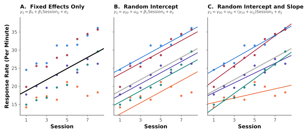
The same data fit with fixed effects, a random intercept, and a random slope

Figure: The three equations above, fit to one simulated dataset of five participants across eight sessions.

The key insight is that random effects are not nuisance parameters to be controlled for. They are the between-person differences that behavior scientists care about. How much do individuals vary in their baseline response rate? How much do they vary in their sensitivity to an intervention? Multilevel models answer these questions directly.

Shrinkage

One of the most elegant features of multilevel models is shrinkage (also called partial pooling). When you estimate a separate mean for each group, groups with little data produce noisy estimates. A participant with only two sessions might appear to have an extremely high or low response rate, but this apparent extremity is partly due to sampling noise.

Multilevel models address this by "shrinking" group-level estimates toward the grand mean. The amount of shrinkage depends on two factors:

How much data the group has: Groups with many observations are shrunk less, because their estimates are more reliable.
How variable groups are overall: If between-group variance is small relative to within-group variance, estimates are shrunk more.

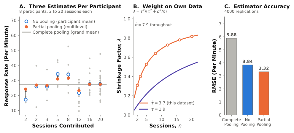
Complete pooling, no pooling, and partial pooling of participant means

Figure: Eight participants contributing 2 to 20 sessions each, estimated three ways.

Shrinkage is not an ad hoc correction. It is a natural consequence of the multilevel model's structure. It is also equivalent to a form of regularization which is the same principle that ridge regression and Bayesian priors use to prevent overfitting. The multilevel model automatically regularizes group-level estimates, producing more accurate predictions than either ignoring groups entirely (complete pooling) or estimating each group independently (no pooling).

This is particularly important for small- $n$ research. Behavior science often works with small numbers of participants, each observed across many sessions. Shrinkage is especially valuable here because it prevents the model parameters from being influenced by extreme data from participants who happen to have fewer or noisier observations.

The Basic Multilevel Equation

The simplest multilevel model is a random-intercept model with no predictors. This is called the unconditional means model or empty model:

y_{ij} = \gamma_{00} + u_{0j} + e_{ij}

where:

$y_{ij}$ is the outcome for observation $i$ in group $j$
$\gamma_{00}$ is the grand mean (the fixed intercept)
$u_{0j}$ is the random intercept for group $j$ , with $u_{0j} \sim N(0, \tau^2)$
$e_{ij}$ is the residual for observation $i$ in group $j$ , with $e_{ij} \sim N(0, \sigma^2)$

This model decomposes each observation into three parts: the overall average, the group's deviation from that average, and the individual observation's deviation from its group average. This is the Level 1 and Level 2 decomposition:

Level 1 (within-person):

y_{ij} = \beta_{0j} + e_{ij}

Level 2 (between-person):

\beta_{0j} = \gamma_{00} + u_{0j}

Substituting the Level 2 equation into Level 1 gives the combined equation above. The beauty of this framework is that it separates within-person variability ( $\sigma^2$ ) from between-person variability ( $\tau^2$ ), and the ICC can be directly computed from these two variance components.

Adding predictors at Level 1 (e.g., session number, condition) and Level 2 (e.g., participant characteristics, treatment group) allows you to explain variance at each level. This is where multilevel models become useful tools for testing hypotheses about individual trajectories and group differences.

Temporal Autocorrelation

In many behavioral datasets, observations are ordered in time, and adjacent observations are correlated. A participant who responds at a high rate in Session 5 is likely to respond at a high rate in Session 6. This phenomenon is temporal autocorrelation.

The autocorrelation function (ACF) quantifies this. For a time series $x_1, x_2, \ldots, x_T$ , the autocorrelation at lag $k$ is the correlation between $x_t$ and $x_{t-k}$ :

\rho_k = \frac{\text{Cov}(x_t, x_{t-k})}{\text{Var}(x_t)}

At lag 0, $\rho_0 = 1$ (a series is perfectly correlated with itself). At lag 1, $\rho_1$ tells you how strongly today's value predicts tomorrow's. At lag 2, $\rho_2$ tells you how strongly today's value predicts the day after tomorrow's. And so on.

In behavioral data, lag-1 autocorrelations are often positive and substantial. Session-to-session response rates, daily self-monitoring data, and within-session interresponse times all tend to show autocorrelation. When autocorrelation is present and ignored, standard errors from ordinary regression are biased, and forecasts fail to exploit the temporal structure of the data.

Plotting the ACF is an essential first step in any time-series analysis. It tells you how much temporal structure exists and suggests what kind of model might be appropriate.

Autoregressive Models AR(p)

The simplest model for temporal dependence is the autoregressive model of order 1, or AR(1):

x_t = \phi \cdot x_{t-1} + \epsilon_t

where:

$x_t$ is the value of the series at time $t$
$\phi$ is the autoregressive coefficient, capturing the magnitude of temporal dependence
$\epsilon_t$ is white noise (independent, identically distributed error), with $\epsilon_t \sim N(0, \sigma^2_\epsilon)$

The AR(1) model says that the current value equals a fraction of the previous value, plus random noise. If $\phi = 0.8$ , then 80% of the current value is "inherited" from the previous time point, and 20% is new random input.

Key properties of AR(1):

If $|\phi| < 1$ , the series is stationary; it fluctuates around a stable mean and does not drift off to infinity.
If $\phi > 0$ , adjacent values tend to be similar (positive autocorrelation). This is the typical case in behavioral data.
If $\phi < 0$ , adjacent values tend to alternate (negative autocorrelation). This is less common but can occur in some behavioral contexts (e.g., contrast effects).
If $\phi = 1$ , the series is a random walk; it drifts without returning to a mean. This is a nonstationary process.

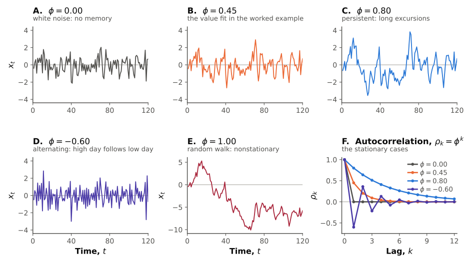
AR(1) series across values of the autoregressive coefficient

Figure: Five AR(1) series generated from the same white noise, varying only $\phi$ .

More generally, an AR(p) model includes $p$ lags:

x_t = \phi_1 \cdot x_{t-1} + \phi_2 \cdot x_{t-2} + \cdots + \phi_p \cdot x_{t-p} + \epsilon_t

AR(2) says the current value depends on the two most recent values. In practice, behavioral time series are often well described by AR(1) or AR(2).

Interpreting $\phi$ in behavioral terms: A high $\phi$ (close to 1) means behavior is highly persistent (i.e., today's response rate is very similar to yesterday's). A low $\phi$ (close to 0) means behavior is relatively unpredictable from one time point to the next. Interventions that aim to disrupt behavioral patterns should, in principle, reduce $\phi$ .

ARIMA Models

ARIMA stands for AutoRegressive Integrated Moving Average. It extends the AR model in two ways:

Differencing (I): If a series has a trend (e.g., response rate gradually increases across sessions), the series is nonstationary. Differencing transforms the series by computing changes: $\Delta x_t = x_t - x_{t-1}$ . This can remove trends and make the series stationary. The "I" in ARIMA indicates how many times differencing is applied.
Moving Average (MA): While AR models regress the current value on past values, MA models regress the current value on past errors:

x_t = \mu + \epsilon_t + \theta_1 \cdot \epsilon_{t-1} + \theta_2 \cdot \epsilon_{t-2} + \cdots + \theta_q \cdot \epsilon_{t-q}

The MA component captures short-lived shocks. If something unusual happened yesterday (a large $\epsilon_{t-1}$ ), the MA term lets that shock influence today's value.

An ARIMA(p, d, q) model combines all three:

$p$ = number of autoregressive terms
$d$ = number of differences needed for stationarity
$q$ = number of moving average terms

For example:

ARIMA(1,0,0) is simply an AR(1) model (no differencing, no MA).
ARIMA(0,1,0) is a random walk (first-differenced series is white noise).
ARIMA(1,1,1) uses one AR term, one difference, and one MA term.

Selecting ARIMA orders: The ACF and partial autocorrelation function (PACF) guide model selection:

An AR(p) process shows a PACF that cuts off after lag $p$ and an ACF that decays gradually.
An MA(q) process shows an ACF that cuts off after lag $q$ and a PACF that decays gradually.
Mixed processes show gradual decay in both.

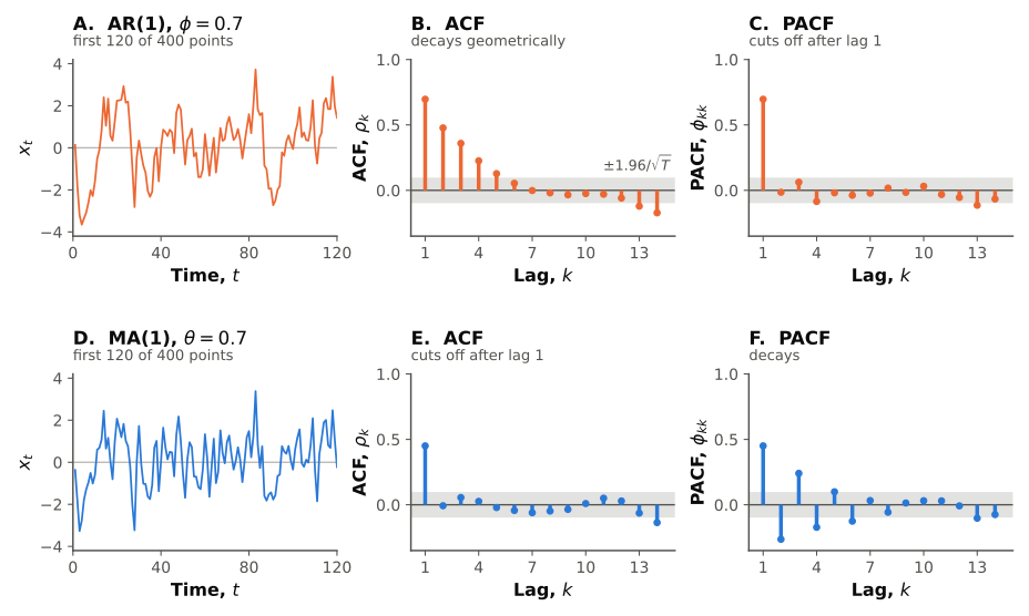
ACF and PACF signatures of AR(1) and MA(1) processes

Figure: The ACF and PACF signatures of an AR(1) and an MA(1) process.

Information criteria (AIC, BIC) are typically used to compare candidate models. The model with the lowest information criterion is preferred, balancing fit against complexity.

ARIMA models are useful for forecasting behavioral time series. That is, predicting tomorrow's response rate from the recent history, projecting the trajectory of a self-monitoring variable, or detecting changes in temporal structure after an intervention.

Time-Series Decomposition

A behavioral time series can often be decomposed into interpretable components:

x_t = T_t + S_t + R_t

where:

$T_t$ is the trend component: the long-term increase or decrease
$S_t$ is the seasonal (or cyclical) component: regular repeating patterns
$R_t$ is the residual (or remainder): what is left after removing trend and seasonality

For example, consider a participant's daily self-monitoring data collected over 90 days. The trend might show a gradual increase in the target behavior over the course of treatment. The seasonal component might reveal a weekly cycle because the participant consistently performs better on weekdays than weekends. The residual captures day-to-day fluctuations that are not explained by trend or cycle.

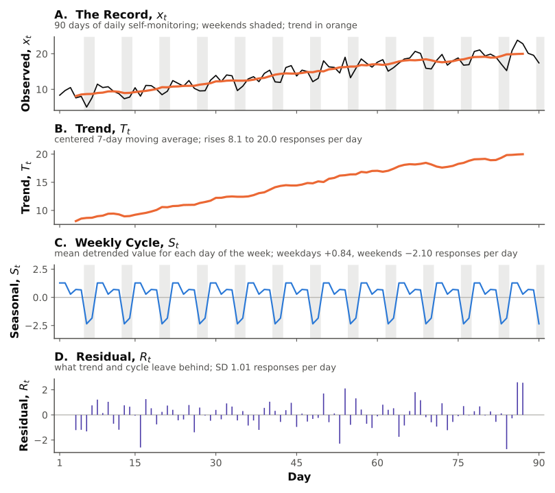
Additive decomposition of a 90-day self-monitoring record

Figure: The 90-day record described above, decomposed additively into $x_t = T_t + S_t + R_t$ .

Decomposition is descriptive rather than inferential, but is still useful. It tells you what the dominant patterns are in your data before you try to build a forecasting model. If there is a trend, you might need differencing. If there is a clear weekly cycle, you might need seasonal terms.

Classical decomposition methods (additive and multiplicative) and more modern approaches (STL: Seasonal and Trend decomposition using Loess) are available. For behavioral data, additive decomposition is typically appropriate unless the amplitude of seasonal fluctuations scales with the level of the series.

Applying the 8-Step Framework

We apply the 8-step framework to a multilevel modeling problem: modeling delay discounting across multiple participants.

Step 1: Identify All Environmental and Behavioral Components of the Phenomenon Delay discounting is the decrease in the subjective value of a reward as the delay to its receipt increases. Participants are asked to choose between smaller-sooner and larger-later rewards across a range of delays. From these choices, we estimate a discounting rate parameter $k$ for each participant. We have data from 20 participants, each completing the task at 6 different delays.

Step 2: Define the Behavioral Principles, Processes, and Intended Scope of the Model We will model how subjective value declines with delay, allowing the discounting rate $k$ to vary across participants. The scope includes both the within-person discounting function and the between-person variability in $k$ . We will not model how discounting develops over time or how it is affected by specific interventions.

Step 3: Write Down the Behavioral Principles, Known Quantitative Laws, and Functional Relationships Mazur's (1987) hyperbolic discounting model:

V = \frac{A}{1 + k \cdot D}

where $V$ is subjective value, $A$ is the amount of the delayed reward, $D$ is the delay, and $k$ is the discounting rate. Higher $k$ means steeper discounting (more impulsive choice).

Step 4: State All Simplifying Assumptions Explicitly

The hyperbolic form adequately describes each individual's discounting.
The parameter $k$ captures stable individual differences.
Log-transformed $k$ values are normally distributed across participants.
Within-person deviations from the hyperbolic function are normally distributed.
All participants experienced the same set of delays and reward amounts.

Step 5: Write the Model Verbally, Then Express It Mathematically Verbally: Each participant's subjective value at a given delay follows a hyperbolic function, but the steepness of discounting varies from person to person. Some people discount steeply (high $k$ ), others shallowly (low $k$ ). We model this variation explicitly.

To linearize for multilevel modeling, we work with $\ln(k)$ and reformulate. One common approach is to estimate $k_j$ for each participant and then model $\ln(k_j)$ at Level 2. But a fully integrated approach fits the nonlinear model with random effects:

Level 1 (within-person):

V_{ij} = \frac{A}{1 + k_j \cdot D_{ij}} + e_{ij}

Level 2 (between-person):

\ln(k_j) = \gamma_0 + u_j, \quad u_j \sim N(0, \tau^2)

In the combined model, each participant has their own discounting rate $k_j$ , which is drawn from a log-normal distribution centered on $\exp(\gamma_0)$ .

Step 6: Verify Dimensional Consistency $V$ is in dollars (or whatever unit the reward is in). $A$ is in dollars. $k$ is in units of inverse time (e.g., 1/days). $D$ is in time units (e.g., days). The product $k \cdot D$ is dimensionless. Thus $\frac{A}{1 + k \cdot D}$ is in dollars. The residual $e_{ij}$ is in dollars. Units are consistent.

Step 7: Specify Starting Values and Constraints $k_j > 0$ for all participants (working on the log scale ensures this). $A$ is known (set by the experimenter). $D$ values are known (set by the experimenter). Starting values for $\gamma_0$ can be based on published norms (e.g., log( $k$ ) values in the range of $-4$ to $0$ are common for monetary discounting with delays in days). The variance $\tau^2$ can be initialized at 1.

Step 8: Check the Math, Test Against Data, and Derive Predictions

Verify: When $D = 0$ , $V = A$ for all participants (no discounting at zero delay). As $D \to \infty$ , $V \to 0$ . These boundary conditions are correct.
Validate: Fit the model to the 20-participant dataset. Examine residuals for systematic patterns. Compare the multilevel model to a model that ignores individual differences (all participants share the same $k$ ) using a likelihood ratio test or information criterion. The multilevel model should fit substantially better if individuals truly differ.
Solve: Given the estimated distribution of $k$ values, predict discounting for a new participant (using the population distribution as a prior), or predict a specific participant's subjective value at an untested delay.

Worked Example

Example A: Multilevel Model for Response Rate Data

Data. Four participants (P1-P4) each complete 5 sessions on a VI schedule. Response rate (responses per minute) is recorded for each session.

Participant	Session 1	Session 2	Session 3	Session 4	Session 5
P1	22	25	23	24	21
P2	38	40	37	41	39
P3	15	18	14	16	17
P4	30	28	32	31	29

Step 1: Compute group means and the grand mean.

$\bar{y}_{P1} = (22+25+23+24+21)/5 = 23.0$
$\bar{y}_{P2} = (38+40+37+41+39)/5 = 39.0$
$\bar{y}_{P3} = (15+18+14+16+17)/5 = 16.0$
$\bar{y}_{P4} = (30+28+32+31+29)/5 = 30.0$
Grand mean: $\bar{y}_{..} = (23.0 + 39.0 + 16.0 + 30.0)/4 = 27.0$

Step 2: Compute the ICC. We need the between-group variance ( $\tau^2$ ) and the within-group variance ( $\sigma^2$ ).

Between-group variance (variance of group means around the grand mean):

\tau^2 = \frac{(23-27)^2 + (39-27)^2 + (16-27)^2 + (30-27)^2}{4-1} = \frac{16 + 144 + 121 + 9}{3} = \frac{290}{3} = 96.67

Within-group variance (average of within-group variances): For P1: $s^2_{P1} = \frac{(22-23)^2+(25-23)^2+(23-23)^2+(24-23)^2+(21-23)^2}{4} = \frac{1+4+0+1+4}{4} = 2.50$

For P2: $s^2_{P2} = \frac{(38-39)^2+(40-39)^2+(37-39)^2+(41-39)^2+(39-39)^2}{4} = \frac{1+1+4+4+0}{4} = 2.50$

For P3: $s^2_{P3} = \frac{(15-16)^2+(18-16)^2+(14-16)^2+(16-16)^2+(17-16)^2}{4} = \frac{1+4+4+0+1}{4} = 2.50$

For P4: $s^2_{P4} = \frac{(30-30)^2+(28-30)^2+(32-30)^2+(31-30)^2+(29-30)^2}{4} = \frac{0+4+4+1+1}{4} = 2.50$

Pooled within-group variance:

\sigma^2 = \frac{2.50 + 2.50 + 2.50 + 2.50}{4} = 2.50

Now compute the ICC:

\text{ICC} = \frac{\tau^2}{\tau^2 + \sigma^2} = \frac{96.67}{96.67 + 2.50} = \frac{96.67}{99.17} = 0.975

Interpretation. The ICC is 0.975. Nearly 98% of the variance in response rate is between participants. Participants differ enormously in their response rates, while within-participant session-to-session variability is small. A multilevel model is clearly warranted.

Step 3: Fit the random-intercept model. The model is:

y_{ij} = \gamma_{00} + u_{0j} + e_{ij}

The estimated parameters are:

$\hat{\gamma}_{00} = 27.0$ (the grand mean response rate)
$\hat{\tau}^2 = 96.67$ (between-participant variance)
$\hat{\sigma}^2 = 2.50$ (within-participant variance)

Step 4: Interpret the random effects. Each participant's estimated intercept is $\hat{\gamma}_{00} + \hat{u}_{0j}$ :

P1: $27.0 + (-4.0) = 23.0$
P2: $27.0 + 12.0 = 39.0$
P3: $27.0 + (-11.0) = 16.0$
P4: $27.0 + 3.0 = 30.0$

With only 4 participants and 5 sessions each, shrinkage is minimal in this example because each group has the same amount of data. In practice, with unbalanced data (some participants having more sessions than others), shrinkage would pull estimates from data-poor participants toward the grand mean.

Step 5: Interpret the fixed effect. The fixed effect $\hat{\gamma}_{00} = 27.0$ is the estimated average response rate across all participants. It represents the "typical" participant in this sample. The variance of random effects ( $\hat{\tau}^2 = 96.67$ ) tells us how much participants vary around this average. The standard deviation of random intercepts is $\sqrt{96.67} \approx 9.83$ , meaning that about 95% of participants' true mean response rates fall within $27.0 \pm 2 \times 9.83$ , or roughly 7.3 to 46.7 responses per minute.

Example B: AR(1) Model for a Single Participant's Time Series

Data. One participant's daily response rate (responses per minute) over 30 days:

Day	Rate	Day	Rate	Day	Rate
1	20.0	11	27.5	21	30.8
2	22.3	12	26.1	22	29.5
3	21.8	13	28.0	23	31.2
4	23.5	14	27.2	24	30.0
5	22.9	15	29.3	25	32.1
6	24.1	16	28.8	26	31.5
7	23.7	17	30.1	27	33.0
8	25.2	18	29.0	28	32.4
9	24.8	19	30.5	29	34.1
10	26.0	20	29.8	30	33.5

The series shows a gradual upward trend and positive autocorrelation---adjacent days have similar values.

Step 1: Check for stationarity. The series has a visible trend (values increase from about 20 to 34 over 30 days). For an AR(1) model, we need stationarity. We can either detrend the series or work with first differences. Let us mean-center and detrend by fitting a linear trend and working with residuals.

The mean is approximately $\bar{x} = 27.7$ . A linear trend yields roughly $x_t \approx 19.5 + 0.47t$ . The detrended residuals $r_t = x_t - (19.5 + 0.47t)$ fluctuate around zero.

Alternatively, we can use first differences: $\Delta x_t = x_t - x_{t-1}$ .

Step 2: Fit the AR(1) model. Working with the detrended residuals, we fit:

r_t = \phi \cdot r_{t-1} + \epsilon_t

Computing the lag-1 autocorrelation of the detrended residuals (which estimates $\phi$ ), we obtain approximately:

\hat{\phi} \approx 0.45

The residual variance is $\hat{\sigma}^2_\epsilon \approx 1.2$ .

Step 3: Interpret $\phi$ . $\hat{\phi} = 0.45$ means that 45% of each day's deviation from trend is "carried over" from the previous day. If the participant had an unusually high day yesterday (positive residual), today's response rate is expected to be somewhat elevated as well, though the effect decays. After two days, the carryover is $0.45^2 = 0.20$ (20%). After three days, $0.45^3 = 0.09$ (9%). The temporal dependence fades quickly.

Step 4: Make a 1-step forecast. Suppose on Day 30, the detrended residual is $r_{30} = 33.5 - (19.5 + 0.47 \times 30) = 33.5 - 33.6 = -0.1$ .

The predicted detrended residual for Day 31 is:

\hat{r}_{31} = \hat{\phi} \cdot r_{30} = 0.45 \times (-0.1) = -0.045

The trend-predicted value for Day 31 is:

\hat{T}_{31} = 19.5 + 0.47 \times 31 = 34.07

The forecast for Day 31 is:

\hat{x}_{31} = \hat{T}_{31} + \hat{r}_{31} = 34.07 + (-0.045) = 34.0

We predict the participant will respond at approximately 34.0 responses per minute on Day 31.

Step 5: Assess uncertainty. The forecast error variance for a 1-step-ahead prediction from an AR(1) model is simply $\sigma^2_\epsilon$ . A 95% prediction interval is approximately:

\hat{x}_{31} \pm 1.96 \times \hat{\sigma}_\epsilon = 34.0 \pm 1.96 \times \sqrt{1.2} = 34.0 \pm 2.15

So the 95% prediction interval for Day 31 is approximately $[31.9, 36.2]$ responses per minute.

Assumptions and Limitations

Multilevel Models

Normality of random effects: The random effects $u_{0j}$ (and $u_{1j}$ , etc.) are assumed to follow a normal distribution. If the true distribution is heavily skewed or bimodal, estimates may be biased. With small numbers of groups, it is difficult to assess this assumption.
Sufficient number of groups: Multilevel models estimate variance components, and variance estimation requires a reasonable number of groups. With fewer than about 10-15 groups (participants), estimates of $\tau^2$ can be unstable. Fixed-effects approaches may be preferred when the number of groups is very small.
Correct specification of random structure: Choosing which effects should be random is a modeling decision. Including too many random effects can lead to convergence problems. Including too few can misattribute between-group variance to within-group variance.
Independence of groups: Multilevel models assume that groups (e.g., participants) are independent of each other after accounting for fixed effects. If participants influence each other (e.g., in group therapy), this assumption is violated.
Linearity: Standard multilevel models assume linear relationships at each level. Nonlinear multilevel models exist (as in the discounting example above) but are more complex to fit and interpret.

Time-Series Models

Stationarity: AR and ARIMA models require the series to be stationary (constant mean and variance over time) or to be made stationary through differencing. Many behavioral time series have trends or changing variance, requiring transformation before modeling.
Linearity: Standard AR and ARIMA models assume linear relationships between current and past values. Nonlinear time-series models exist (threshold AR, regime-switching models) but are more complex.
Sufficient time points: Time-series models require enough observations to estimate temporal structure reliably. A rule of thumb for ARIMA modeling is at least 30-50 time points. Many behavioral studies have fewer sessions than this, limiting the applicability of pure time-series methods.
Single-subject focus: Traditional time-series models are fit to one individual's data. Extending them to multiple individuals requires either fitting separate models to each person (losing the ability to pool information across individuals) or embedding them within a multilevel framework (adding complexity).
Choosing model orders: Selecting $p$ , $d$ , and $q$ for ARIMA is partly art and partly science. Automatic selection algorithms (e.g., auto.arima) help, but they are not infallible. Model misspecification can lead to poor forecasts.
Assumption of equal spacing: Standard time-series models assume observations are equally spaced in time. Missing sessions or irregular scheduling can cause problems that require specialized methods.

Connection to Empirical Behavior Science

Young (2018) applied multilevel models to choice data, demonstrating how individual differences in sensitivity to reinforcer amount and delay could be captured within a hierarchical framework. This work showed that ignoring nesting in choice datasets led to systematically different (and less accurate) conclusions about the determinants of choice.

Peugh (2010) provided a practical guide to multilevel modeling that has been widely cited in the behavioral and educational sciences. The paper walks through the logic of random effects, ICC computation, and model building in accessible terms, making it an excellent companion to this week's material.

Cox and Vladescu (2023) examined time-series decomposition applied to behavioral data, showing how trend, seasonal, and residual components could be separated in repeated behavioral observations. This work demonstrated that behavioral data often contain temporal structure that standard analyses miss, and that decomposition can reveal patterns relevant to treatment evaluation.

Adhikari and Agrawal (2013) reviewed forecasting methods including ARIMA and its extensions, providing a broad overview of time-series approaches applicable to behavioral and social science data. Their comparison of forecasting accuracy across methods provides useful guidance for selecting among candidate time-series models.

These references collectively illustrate that both multilevel and time-series methods are not just abstract statistical tools. Each of these models are actively being used in behavior science to answer substantive questions about behavioral processes.

Exercises for Reflection

ICC and study design: Suppose you are planning a study in which you will measure the number of problem behaviors per session for children in a special education classroom. You expect substantial variability across children but relatively little variability across sessions within a child (ICC around 0.70). How does this high ICC affect the effective sample size of your study? Would adding more sessions per child or more children do more to increase statistical power?
Random slopes: Consider a study examining how an intervention affects response rate across sessions. You fit a random-intercept model and a random-intercept-random-slope model (where the slope of session number is allowed to vary across participants). What would it mean, substantively, if the random slope variance is large? What would it mean if it is near zero? How would you decide which model to use?
Interpreting autocorrelation: You collect daily data on a client's self-injurious behavior over 60 days. The ACF shows a strong lag-1 autocorrelation of 0.7, with autocorrelations at higher lags decaying gradually. What does this pattern suggest about the temporal dynamics of the behavior? What kind of time-series model would be appropriate? How might you use this model clinically?
Combining approaches: Imagine you have daily response rate data for 15 participants over 30 days each. You want to model both individual differences in average response rate and temporal autocorrelation within each person's series. Describe, conceptually, how you might combine multilevel modeling and time-series modeling to address both features of the data simultaneously. What would the model need to include?

Key Readings

Required: Peugh (2010) provided a practical, step-by-step guide to multilevel modeling for researchers in education and psychology, covering the rationale for multilevel analysis, the intraclass correlation coefficient, random intercepts and slopes, and model-building strategies. He demonstrated why ignoring nested data structure leads to inflated Type I error rates and showed how multilevel models correct this by partitioning variance into within-group and between-group components. This paper is the methodological backbone of the week's first topic: it gives students the conceptual and practical tools to handle the hierarchical data structures that are ubiquitous in behavior science (e.g., trials within sessions, sessions within participants).

Young (2018) applied the multilevel modeling framework specifically to delay discounting data, showing how to fit nonlinear discounting functions within a hierarchical structure that accounts for individual differences in discounting parameters. He demonstrated that the multilevel approach is superior to the traditional method of fitting each participant separately because it pools information across individuals, handles sparse data gracefully, and allows researchers to model covariates of individual differences in a single integrated analysis. This paper connects the week's statistical methodology directly to a model students already know (e.g., hyperbolic discounting from Week 2) showing that the tools from this week enhance rather than replace the models from earlier weeks.

Cox and Vladescu (2023) introduced time-series decomposition and forecasting methods for behavioral data, covering trend extraction, seasonal components, autoregressive models, and ARIMA. They demonstrated how these techniques can be applied to the kind of repeated within-subject observations that characterize applied behavior analysis, enabling practitioners to forecast future behavior and detect changes in level or trend that signal treatment effects. This chapter addresses the temporal-dependence side of the week's content: where multilevel models handle the between-person nesting, time-series methods handle the within-person sequential structure that makes today's observation depend on yesterday's.

Supplemental: Quene and van den Bergh (2004) provided a tutorial on multilevel modeling for repeated-measures designs, using examples from speech and communication research to illustrate the advantages over traditional repeated-measures ANOVA. They emphasized the flexibility of multilevel models in handling unbalanced designs, missing data, and continuous time variables; each are features that make the approach particularly well suited to behavioral datasets, where participants often contribute different numbers of sessions and missing data are common. This paper reinforces the week's core message from a different disciplinary angle, helping students see that the multilevel framework is a general-purpose tool, not a domain-specific technique.

Adhikari and Agrawal (2013) provided a broad introduction to time-series modeling and forecasting, covering the mathematical foundations of stationarity, autocorrelation, ARIMA models, and model selection criteria. They presented the material with an emphasis on practical implementation, including step-by-step procedures for model identification, estimation, and diagnostic checking. This paper complements the Cox and Vladescu chapter by providing deeper mathematical detail on the time-series methods, giving students who want to move beyond the applied primer a more rigorous treatment of the underlying theory.

Reading Guide

Peugh (2010)

What is multilevel modeling (MLM), and why is it necessary when data have a nested structure?
What are "levels" in a multilevel model? Give a behavioral example with at least two levels.
What is the intraclass correlation coefficient (ICC), and what does it tell you about the data structure?
At what ICC value does ignoring the nesting become problematic? Why?
What is the difference between a fixed effect and a random effect in a multilevel model?
What is a random intercept model? What behavioral question does it answer?
What is a random slope model? When would you need random slopes in addition to random intercepts?
How does MLM handle unbalanced data (different numbers of observations per unit)? Why is this advantage important for behavioral research?
What assumptions does MLM make about the distribution of random effects?
How do you determine whether adding a random effect improves the model? What test is used?
What is the difference between Level-1 and Level-2 predictors? Give a behavioral example of each.
Why does Peugh argue that ordinary least squares (OLS) regression is inappropriate for nested data?
What happens to standard errors and p-values when nesting is ignored? Why is this a problem?
How does MLM relate to repeated-measures ANOVA? What advantages does MLM offer?
What practical recommendations does Peugh provide for researchers new to multilevel modeling?

Young (2018)

How does Young apply multilevel modeling specifically to delay discounting data?
Why is discounting data inherently multilevel (what are the levels)?
What are the advantages of fitting discounting models within a multilevel framework compared to fitting each participant separately?
How does the multilevel approach handle participants with sparse or noisy data?
What is a nonlinear multilevel model, and why is it needed for discounting data?
How does the multilevel framework allow researchers to examine individual differences in discounting parameters?
What covariates can be included at the participant level, and how does this extend the analysis beyond simple curve fitting?
What practical guidance does Young offer for implementing multilevel discounting analyses?
How does this approach compare to the traditional method of estimating $k$ for each participant and then analyzing the $k$ values?
What are the limitations of the multilevel approach as discussed by Young?

Cox & Vladescu (2023)

What is time-series decomposition, and what are the components of a time series?
What is the difference between trend, seasonality, and residual components?
Why is it important to decompose a behavioral time series before modeling it?
What is stationarity, and why does it matter for time-series analysis?
How do you test whether a behavioral time series is stationary?
What is an autoregressive (AR) model, and what does the autoregressive parameter tell you about behavior?
What is the difference between AR, MA, and ARIMA models?
How can time-series methods be applied to single-case behavioral data?
What are some practical applications of time-series forecasting in behavior analysis?
How do the authors suggest interpreting autocorrelation in behavioral data?

References

Adhikari, R., & Agrawal, R. K. (2013). An introductory study on time series modeling and forecasting. arXiv. https://doi.org/10.48550/arXiv.1302.6613

Cox, D. J., & Vladescu, J. C. (2023). Statistics for applied behavior analysis practitioners and researchers. Academic Press.

Mazur, J. E. (1987). An adjusting procedure for studying delayed reinforcement. In M. L. Commons, J. E. Mazur, J. A. Nevin, & H. Rachlin (Eds.), Quantitative analyses of behavior: Vol. 5. The effect of delay and of intervening events on reinforcement value (pp. 55--73). Erlbaum.

Peugh, J. L. (2010). A practical guide to multilevel modeling. Journal of School Psychology, 48(1), 85--112. https://doi.org/10.1016/j.jsp.2009.09.002

Quené, H., & van den Bergh, H. (2004). On multi-level modeling of data from repeated measures designs: A tutorial. Speech Communication, 43(1--2), 103--121. https://doi.org/10.1016/j.specom.2004.02.004

Young, M. E. (2018). Discounting: A practical guide to multilevel analysis of choice data. Journal of the Experimental Analysis of Behavior, 109(2), 293--312. https://doi.org/10.1002/jeab.316

Key Takeaways

Nested data require multilevel models. When observations are grouped (e.g., sessions within participants), treating them as independent inflates Type I error. Multilevel models decompose variance into within-group and between-group components.
The ICC tells you how much nesting matters. ICC = $\tau^2 / (\tau^2 + \sigma^2)$ . When ICC is nontrivial, you need a multilevel model.
Random effects capture individual differences. Random intercepts allow each participant to have their own baseline. Random slopes allow the effect of a predictor to vary across participants. These are not nuisance parameters---they are often the quantities of greatest scientific interest.
Shrinkage is automatic regularization. Multilevel models pull extreme estimates from data-poor groups toward the grand mean, producing more accurate predictions than either pooled or unpooled approaches.
Temporal autocorrelation is the norm in behavioral data. Adjacent observations tend to be correlated. The ACF quantifies this structure.
AR(1) is the simplest time-series model. $x_t = \phi \cdot x_{t-1} + \epsilon_t$ . The parameter $\phi$ captures the magnitude of temporal persistence.
ARIMA extends AR to handle trends and shocks. ARIMA(p,d,q) combines autoregressive terms, differencing, and moving average terms. It is the workhorse of time-series forecasting.
Time-series decomposition separates trend, seasonality, and noise. This is a crucial descriptive step before building a forecasting model.
Together, multilevel and time-series models address the two fundamental structures in behavioral data: people are different from each other, and behavior unfolds over time.