Week 8: Probability Theory and Probabilistic Models

Why This Topic Matters

Real behavioral data are noisy. Response rates fluctuate from session to session, interresponse times vary from one response to the next, and measurement itself introduces error. If you record the same organism responding to the same reinforcement schedule for 30 consecutive sessions, you will get 30 different response rates. This variability is not a flaw in the experiment but a feature of complicated and complex phenomena.

Most of the models introduced so far in this course have been deterministic. Given values for the independent variables and parameters, the model produces a single predicted value. $R = k \cdot t$ predicts exactly 60 responses in 30 minutes if $k = 2$ . But the observed count will almost never be exactly 60. Something is missing.

Probabilistic models help fill this gap. Instead of predicting a single value, probabilistic models predict a distribution of possible values, each with an associated probability. Using the example above, the model does not predict exactly 60 responses. Rather, it predicts the expected number of responses to be 60 and the probability of observing between 55 and 65 as, say, 0.73. The idea is to be precise about uncertainty when making predictions.

Probability theory provides the mathematical foundation for three activities that are central to modeling:

Parameter estimation: When you fit a model to data, you need a criterion for choosing the best parameter values. Maximum likelihood estimation is the most widely used method and is built on probability theory.
Hypothesis testing and model comparison: When you ask whether Model A describes data better than Model B, the answer depends on the probability of the data under each model.
Understanding behavioral variability: Variability is not just noise we can average away. That noise can be explained as the result of the complex multiple control of behavior. But, when the full deterministic influence of relevant variables is unknown, probabilistic models improve our ability to make accurate predictions.

This week introduces the core ideas in probability theory of random variables, probability distributions, conditional probability, Bayes' theorem, maximum likelihood estimation, and signal detection theory. These will appear repeatedly in subsequent weeks.

Core Concepts

Random Variables and Distributions

A random variable is a numerical quantity whose value is determined by the outcome of a random process. When a rat presses a lever, the interresponse time (IRT) (i.e., the time between one press and the next) can be modeled as a random variable.

A probability distribution describes how likely each possible value (or range of values) of a random variable is. For a discrete random variable (one that takes on countable values), the distribution assigns a probability to each value. For a continuous random variable, the distribution is described by a probability density function (PDF), and probabilities correspond to areas under the curve.

There are three distributions that are especially important for behavior science. The first is the binomial distribution which models the number of successes in a fixed number of independent trials, each with the same probability of success. If a pigeon pecks a key on each of 20 trials, and the probability of pecking on any given trial is $p$ , then the number of pecks across trials follows a binomial distribution:

P(k) = \binom{n}{k} p^k (1-p)^{n-k},

where $n$ is the number of trials and $k$ is the number of successes. The arithmetic mean of the binomial is $np$ and the variance is $np(1-p)$ .

The binomial distribution is useful for modeling phenomena such as discrete-trial procedures, choice proportions, and any situation where each observation is a binary outcome. In a matching-to-sample task with 20 trials, if the organism has a true probability of 0.80 of selecting the correct comparison, the binomial distribution tells you the probability of observing any particular number of correct trials. For instance, the probability of getting exactly 16 correct is $\binom{20}{16}(0.8)^{16}(0.2)^4 \approx 0.218$ .

The second distribution important to behavior science is the Poisson distribution. The Poisson distribution models the number of events occurring in a fixed interval of time (or space), given a constant average rate. If lever presses occur at an average rate of $\lambda$ per minute, then the probability of observing exactly $k$ presses in one minute is:

P(k) = \frac{\lambda^k \cdot e^{-\lambda}}{k!}.

The Poisson distribution has a single parameter, $\lambda$ , which is both the mean and the variance. Claiming that the mean equals variance is a testable prediction. If you observe response counts with a mean of 10 but a variance of 30, the Poisson model is telling you that the data are more variable than random events at a constant rate would produce (i.e., something is producing time-varying rates and should be sussed out).

The Poisson distribution is the workhorse for modeling count data in behavior science such as responses per interval, reinforcers delivered per session, or problem behaviors per observation period. If conditions are functionally constant, the Poisson distribution should describe phenomena like these well. For example, if an organism produces an average of 4 responses per minute, the Poisson model predicts $P(0) = e^{-4} \approx 0.018$ , $P(4) \approx 0.195$ , and $P(8) \approx 0.030$ . The distribution is right-skewed for small $\lambda$ and becomes approximately symmetric as $\lambda$ increases.

The third important distribition ia the normal (Gaussian) distribution. The Gaussian distribution describes continuous measurements that cluster symmetrically around a mean. It is characterized by the two parameters of the mean $\mu$ and the variance $\sigma^2$ :

f(x) = \frac{1}{\sqrt{2\pi\sigma^2}} \exp\left(-\frac{(x - \mu)^2}{2\sigma^2}\right).

The normal distribution arises when a measurement is the sum of many small, independent influences (the central limit theorem). It is often the default assumption for measurement error in many modeling contexts and the foundation for much of classical statistics.

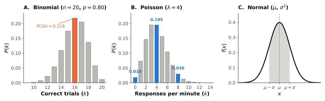
The three distributions used most often in behavior science

Figure: The three distributions using the values worked in the text.

The central limit theorem is the reason the normal distribution appears so often in mathematical modeling. The central limit theorem states that if you average many independent random quantities, the average will be approximately normally distributed regardless of the distribution of the individual quantities. This means that session-level averages (mean response rate across many intervals, mean latency across many trials) will tend to be approximately normal even if the individual observations are not.

With the above in mind, a natural question is how you decide which distribution to use? Fortunately, you do not have to know this beforehand as the data will determine this choice. If the data are counts of events in fixed intervals, start with the Poisson. If the data are proportions from a fixed number of trials, start with the binomial. If the data are continuous measurements that can be positive or negative, start with the normal. If the data are durations or waiting times, the exponential or gamma distributions are natural candidates. The choice of distribution is a modeling decision that should be justified and checked against the data.

The Poisson Process

The Poisson process is a model for events occurring randomly in time at a constant average rate. It is one of the simplest and most useful stochastic models in behavior science.

Definition. A Poisson process with rate $\lambda$ has three defining properties:

Events occur one at a time (no simultaneous events).
The number of events in non-overlapping intervals is independent.
The probability of an event in a short interval of length $\Delta t$ is approximately $\lambda \Delta t$ .

From these properties, two key results follow: Count distribution. The number of events in an interval of length $t$ follows a Poisson distribution with parameter $\lambda t$ :

P(k \text{ events in } t) = \frac{(\lambda t)^k \cdot e^{-\lambda t}}{k!}.

Inter-event time distribution. The time between consecutive events follows an exponential distribution with rate $\lambda$ :

f(\tau) = \lambda e^{-\lambda \tau}, \quad \tau \geq 0.

The mean inter-event time is $1/\lambda$ and the variance is $1/\lambda^2$ .

The Poisson process is the simplest model for the timing of operant responses. If a rat presses a lever at an average rate of 10 presses per minute, and if those presses are well modeled by a Poisson process, then the IRTs should follow an exponential distribution with mean $1/10 = 0.1$ minutes (6 seconds). The number of presses in any 1-minute bin should follow a Poisson distribution with $\lambda = 10$ .

The Poisson process also describes the reinforcement schedule itself in a variable-interval (VI) arrangement. A VI 60-s schedule arranges reinforcers according to a Poisson process with $\lambda = 1/60$ reinforcers per second (or 1 per minute).

And example may help. Suppose a pigeon emits $\lambda = 0.5$ responses per second (30 responses per minute). The mean IRT is $1/0.5 = 2$ seconds. The probability of an IRT exceeding 5 seconds is $P(\tau > 5) = e^{-0.5 \times 5} = e^{-2.5} \approx 0.082$ , or about 8%. The probability of an IRT exceeding 10 seconds is $P(\tau > 10) = e^{-5} \approx 0.007$ , less than 1%. Long pauses are possible but rare under the Poisson model.

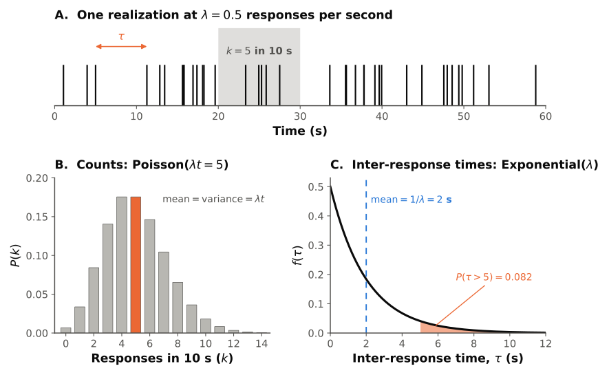
Counts and inter-response times under a Poisson process

Figure: Panel A is a 60-s Poisson process at $\lambda = 0.5$ responses per second, with each response drawn as a tick and one inter-response time ( $\tau$ ) marked. Counting responses in a fixed interval yields the Poisson distribution (B), whose mean and variance are both $\lambda t$ ; measuring the gaps between responses yields the exponential distribution (C), whose mean is $1/\lambda = 2$ s and whose tail beyond 5 s holds 8% of inter-response times. The shaded window in A contains 5 responses, which is the count the distribution in B predicts on average.

The exponential distribution has a unique property called memorylessness defined as $P(\tau > s + t | \tau > s) = P(\tau > t)$ . In words, if an organism has not responded for $s$ seconds, the probability of responding in the next $t$ seconds is the same as if no time had passed. This assumption means there is no increased in the probability of responding as time increases since the last response. The organism is equally likely to respond in the next second regardless of how long it has been since the last response.

The Poisson process assumes a constant rate of responding and, thus, fails when this assumption is not met. For example, response rates might change within a session due to temporal carryover, satiation, or local schedule effects. As another example, post-reinforcement pauses on ratio schedules also violate the constant-rate assumption. And, response bursts (i.e., clusters of very rapid responses) violate the constant-rate and independence assumptions.

When the rate is not constant, more complex models are needed. For example, an inhomogeneous Poisson process allows $\lambda$ to vary as a function of time: $\lambda(t)$ ; a mixture model posits two or more states (e.g., "engaged" and "disengaged"), each with its own rate that the organism switches between; and renewal process drops the memorylessness assumption, allowing the hazard of a response to depend on the time since the last response. Each of these (and other) extensions are built on the Poisson process as a foundation, which is why understanding the simple case is essential.

Conditional Probability and Bayes' Theorem

Conditional probability is the probability of one event given that another event has occurred. The notation $P(A|B)$ is read "the probability of $A$ given $B$ ." It is defined as:

P(A|B) = \frac{P(A \cap B)}{P(B)},

where $P(A \cap B)$ is the probability that both $A$ and $B$ occur, and $P(B) > 0$ .

Conditional probability is everywhere in behavior science. The probability that an organism responds given that a stimulus is present is a conditional probability and often described as the "strength" of stimulus control. The probability that a behavior is maintained by attention given that attention follows the behavior is another example of a conditional probability.

Bayes' theorem relates conditional probabilities in a way that allows us to invert them. That is, to go from $P(\text{data}|\text{hypothesis})$ to $P(\text{hypothesis}|\text{data})$ :

P(H|D) = \frac{P(D|H) \cdot P(H)}{P(D)},

where:

$P(H|D)$ is the posterior probability (i.e., our updated belief about the hypothesis after seeing the data).
$P(D|H)$ is the likelihood (i.e., the probability of the data if the hypothesis is true).
$P(H)$ is the prior probability (i.e., our belief about the hypothesis before seeing the data).
$P(D)$ is the marginal likelihood or evidence (i.e., the total probability of the data across all hypotheses).

An example may help. Suppose you are conducting a functional analysis and you want to know whether a child's problem behavior is maintained by escape from demands. Before collecting data, you assign a prior probability of $P(\text{escape}) = 0.30$ based on the literature on functional analysis outcomes and interview with caregivers. You then observe elevated rates of problem behavior in a single escape condition relatie to a single control condition. The questions are how much should this observation change your belief, and should you run more sessions?

Bayes' theorem provides a quantitative answer. The likelihood $P(\text{elevated rates}|\text{escape function})$ might be high (say, 0.85), because if escape truly maintains the behavior, elevated rates in the escape condition are expected. The likelihood under the alternative $P(\text{elevated rates}|\text{not escape})$ might be lower (say, 0.20), because elevated rates could occur for other reasons but this would be less frequent.

We can compute the posterior explicitly. Using the full form of Bayes' theorem:

P(\text{escape}|\text{elevated}) = \frac{P(\text{elevated}|\text{escape}) \cdot P(\text{escape})}{P(\text{elevated})}

The denominator $P(\text{elevated})$ is computed by the law of total probability:

P(\text{elevated}) = P(\text{elevated}|\text{escape}) \cdot P(\text{escape}) + P(\text{elevated}|\text{not escape}) \cdot P(\text{not escape})

= (0.85)(0.30) + (0.20)(0.70) = 0.255 + 0.140 = 0.395.

Therefore:

P(\text{escape}|\text{elevated}) = \frac{(0.85)(0.30)}{0.395} = \frac{0.255}{0.395} \approx 0.645

The observation of elevated rates has doubled the probability of an escape function from 0.30 (the prior) to 0.645 (the posterior). This is why Bayes' theorem is useful. It tells you exactly how much a newly collected datumshould change your belief, given your prior state of knowledge and the diagnosticity of the evidence. And, it's easy to see how your beliefs can be updated constantly over time to capture things like the changing function of behavior and novel stimulus control.

Bayesian Updating

Bayesian updating is the iterative application of Bayes' theorem as new data arrive. It provides a formal model of how rational belief revision works.

The process is straightforward:

Start with a prior distribution over the parameter or hypothesis of interest. This represents your state of knowledge before collecting data.
Observe data and compute the likelihood of the data under each possible parameter value.
Apply Bayes' theorem to obtain the posterior distribution.
The posterior becomes the new prior distribution when the next batch of data arrives.

This iterative structure means that Bayesian updating naturally accumulates evidence. Early in a study, when little data are available, the posterior is strongly influenced by the prior. As data accumulate, the likelihood dominates, and the posterior concentrates around the parameter value best supported by the evidence.

Formally, this an be stated as: if $\theta$ is a parameter with prior distribution $p(\theta)$ , and we observe data $D$ , the posterior distribution is:

p(\theta|D) = \frac{p(D|\theta) \cdot p(\theta)}{p(D)},

where $p(D) = \int p(D|\theta) \cdot p(\theta) \, d\theta$ is the normalizing constant.

Bayesian updating is sometimes described as a model of learning from evidence. An organism (or a clinician, or a researcher) starts with some expectation about the world, encounters new information, and updates (i.e., learns). The mathematics ensures that the update is calibrated such that strong evidence produces large shifts, weak evidence produces small shifts, and the certainty of the updated belief reflects the quantity and quality of the total evidence to date.

Several computational models of animal learning are explicitly Bayesian (e.g., Kalman filter models of classical conditioning). That is, the organism is modeled as maintaining and updating a probability distribution over the state of the environment.

Given the mathematical update mechanism, an interesting question arises as to how much data one needs before their estimates are likely to be accurate. With very little data, the posterior is dominated by the prior. With a lot of data, the posterior is dominated by the likelihood, and the prior becomes irrelevant. This means that two researchers who start with different priors will converge on the same posterior given enough data. The prior matters most when data are scarce, which is precisely when we need it most, because without some starting point, we cannot make any inference at all.

There are several strategies to choose a prior distribution in practice. One method is to choose uninformative (flat) priors to assume maximal ignorance. The uniform distribution Beta(1,1) is the standard example for an uninformative prior probability distribution. A second method is to use weakly informative priors that constrain the parameter to plausible ranges without placing a high probability on any particular value. For example, Beta(2,2) puts slightly more weight near 0.5 than at the extremes. A third approach is to choose informative priors which incorporate specific prior knowledge, such as results from previous studies or theoretical constraints. Lastly, and most ideal, is to use empirical priors which are estimated from data (e.g., from a separate sample or from the literature). The choice of prior should be documented and its influence assessed via sensitivity analysis.

Maximum Likelihood Estimation (MLE)

Maximum likelihood estimation is the most widely used method for fitting models to data. The idea is simply to choose the parameter values that make the observed data most probable. This is done using the likelihood function. Given a model with parameter(s) $\theta$ and observed data $x_1, x_2, \ldots, x_n$ , the likelihood function is:

L(\theta | \text{data}) = \prod_{i=1}^{n} P(x_i | \theta).

This is the joint probability of all observed data, treated as a function of $\theta$ . Note the difference from ordinary probability where $\theta$ is fixed and we compute the probability of data. In likelihood, the data are fixed and we evaluate different values of $\theta$ .

The maximum likelihood estimate is the value $\hat{\theta}$ that maximizes $L(\theta|\text{data})$ :

\hat{\theta} = \arg\max_\theta L(\theta | \text{data}).

In practice, it is common to use the log-likelihood because products become sums and the computations are more stable:

\ell(\theta | \text{data}) = \sum_{i=1}^{n} \ln P(x_i | \theta).

Maximizing the log-likelihood gives the same answer as maximizing the likelihood (because the logarithm is a monotonically increasing function).

An example may help. Suppose you observe the following counts of lever presses in five successive 1-minute bins: 8, 12, 7, 11, 9. You assume a Poisson model with rate $\lambda$ . The log-likelihood is:

\ell(\lambda) = \sum_{i=1}^{5} \left[ k_i \ln \lambda - \lambda - \ln(k_i!) \right].

Taking the derivative with respect to $\lambda$ , setting it equal to zero, and solving yields:

\hat{\lambda} = \frac{1}{n} \sum_{i=1}^{n} k_i = \frac{8 + 12 + 7 + 11 + 9}{5} = \frac{47}{5} = 9.4.

The MLE of a Poisson rate is the sample mean. This is intuitive, but the MLE framework gives us much more than just the estimate. MLE also gives us the full likelihood surface from which we can derive confidence intervals, conduct hypothesis tests, and compare models.

It's important to explicitly note that likelihood is not probability. This distinction trips up many people. The probability $P(x|\theta)$ is a probability distribution over $x$ for fixed $\theta$ . $P(x|\theta)$ sums (or integrates) to 1 over $x$ . The likelihood $L(\theta|x)$ is a function of $\theta$ for fixed $x$ : it does not necessarily sum or integrate to 1 over $\theta$ . Likelihood tells you how well each parameter value accounts for the data, but it is not a probability distribution over parameters. (Bayesian inference converts likelihood into a probability distribution over parameters by multiplying by a prior and normalizing.)

An analogy may help. Consider a detective evaluating suspects. The likelihood of suspect A given the evidence is a measure of how well suspect A explains the evidence. The likelihood of suspect B is a measure of how well suspect B explains the evidence. These likelihoods are useful for comparing suspects, but they are not probabilities as they do not sum to 1 across all suspects, and they do not directly tell you the probability that suspect A committed the crime. To get that probability, you would need prior information (base rates, alibis) combined with the likelihood, which is what Bayes' theorem does.

In large samples, maximum likelihood estimators have several desirable properties:

Consistency: As sample size increases, $\hat{\theta}$ converges to the true value of $\theta$ .
Asymptotic normality: The distribution of $\hat{\theta}$ around the true value becomes approximately normal.
Efficiency: Among all consistent estimators, the MLE achieves the smallest possible variance (asymptotically).
Invariance: If $\hat{\theta}$ is the MLE of $\theta$ , then $g(\hat{\theta})$ is the MLE of $g(\theta)$ for any function $g$ .

These properties make MLE the default estimation method in most modeling contexts, including the behavioral models covered in this course.

Signal Detection Theory

Signal detection theory (SDT) provides a framework for analyzing decisions made under uncertainty. Specifically, decisions about whether a signal is present or absent when the evidence is noisy.

SDT experiments usually have a very basi setup. On each trial, an observer decides whether a signal was present (e.g., "the child engaged in the target behavior") or absent ("the child did not engage in the target behavior"). The observer's sensory or perceptual evidence varies from trial to trial. On signal-present trials, the evidence tends to be higher; on signal-absent trials, it tends to be lower. But the distributions overlap, so the observer cannot be certain.

There are, thus, four outcomes that might occur on any trial:

	Signal Present	Signal Absent
Observer says "yes"	Hit	False Alarm
Observer says "no"	Miss	Correct Rejection

Two quantitative measures are often derived from these data. The first is sensitivity ( $d'$ ) which measures the observer's ability to discriminate signal from noise. It is the distance between the means of the signal and noise distributions, measured in standard deviation units:

d' = z(\text{Hit Rate}) - z(\text{False Alarm Rate}),

where $z$ is the inverse of the standard normal cumulative distribution function. Higher $d'$ means better discrimination.

The second is criterion ( $c$ ) which measures the observer's response bias. That is, their tendency to say "yes" regardless of whether the signal is present. It is calculated as:

c = -\frac{1}{2}\left[z(\text{Hit Rate}) + z(\text{False Alarm Rate})\right].

A criterion of zero indicates no bias; a positive criterion indicates a conservative bias (tendency to say "no"); a negative criterion indicates a liberal bias (tendency to say "yes").

There are numerous applications of SDT in behavior science. For example, when a human observer watches a video and records whether a behavior occurred during each interval, the observer is performing a signal detection task. Reliability between observers can be analyzed using SDT, separating genuine differences in sensitivity from differences in response bias. Two observers might have identical sensitivity ( $d'$ ) but different criteria, leading to different rates of "behavior present" scoring.

Discrimination tasks offer a second set of examples. In a conditional discrimination procedure, an organism must respond differently in the presence of different stimuli. SDT provides a framework for analyzing discrimination performance that separates sensitivity (how well the organism discriminates the stimuli) from bias (the organism's overall tendency to respond to one alternative).

A final example is with clinical decision-making. When a clinician decides whether an assessment result indicates the presence of a condition, SDT applies. A functional analysis that correctly identifies escape-maintained behavior is a "hit". A functional analysis that indicates escape maintenance when the behavior is actually maintained by attention is a "false alarm". SDT helps evaluate the diagnostic accuracy of assessment procedures.

We can convert all of these into a numerical example. Suppose an observer watching video clips has a hit rate of 0.85 and a false alarm rate of 0.15. Then:

$d' = z(0.85) - z(0.15) = 1.04 - (-1.04) = 2.08$ , and

c = -\frac{1}{2}[z(0.85) + z(0.15)] = -\frac{1}{2}[1.04 + (-1.04)] = 0.

This observer has good sensitivity ( $d' = 2.08$ ), indicating strong discrimination between signal and noise. And, they also display no response bias ( $c = 0$ ). Now consider a second observer with a hit rate of 0.85 and a false alarm rate of 0.40. For them:

$d' = z(0.85) - z(0.40) = 1.04 - (-0.25) = 1.29$ , and

c = -\frac{1}{2}[1.04 + (-0.25)] = -0.395.

This observer has lower sensitivity ( $d' = 1.29$ ) and a bias towards saying, "yes" ( $c = -0.395$ ). The two observers might have similar overall accuracy rates, but their underlying performance is quite different. SDT reveals this; simple agreement statistics do not.

You can likely imagine that reinforcement and punishment contingencies will influence responding toward yes or no. By varying the criterion (e.g., instructing observers to be more or less conservative, signaling differential reinforcment in one direction or the other), a researcher or practitioner can trace out a Receiver Operating Characteristic (ROC) curve which is a plot of hit rate versus false alarm rate. An observer with perfect sensitivity would produce a point at (0, 1) on this plot. An observer who is guessing would fall along the diagonal. The area under the ROC curve (AUROC) is a criterion-free measure of sensitivity and is widely used in diagnostic testing.

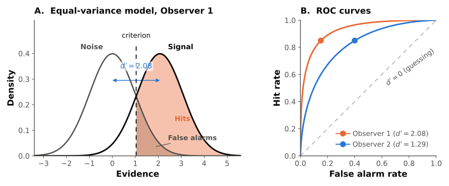
Sensitivity, criterion, and the ROC curve

Figure: Signal detection theory for the two observers described above.

Applying the 8-Step Framework

This section walks through each step of the 8-step modeling framework for modeling the timing of lever presses as a Poisson process for a rat responding on a VI 60-s schedule of food reinforcement.

Step 1: Identify All Environmental and Behavioral Components of the Phenomenon A food-deprived rat is placed in an operant chamber with a single lever. Presses on the lever contact reinforcement with food pellets on a VI 60-s schedule. After 40+ sessions at this schedule value, the rat's responding has reached a steady state. We are interested in the temporal distribution of lever presses within a session. Specifically, we want to model when lever presses occur, not just the overall rate.

Observing the data, we note that the rat presses at a roughly constant rate of about 15 responses per minute during the middle portion of sessions. The IRTs are variable with some being very short (rapid bursts) and others are longer. When we plot a histogram of IRTs, we see a distribution that is roughly exponential with many short IRTs and progressively fewer long ones, with a long right tail. This pattern is consistent across sessions, suggesting a stable underlying process that we can attempt to model.

The key observation driving our modeling decision is that the responses look random. There is no obvious periodicity, no predictable pattern in when each press occurs. This randomness is is the phenomenon we want to capture.

Step 2: Define the Behavioral Principles, Processes, and Intended Scope of the Model We will model the emission of lever presses during steady-state performance in the middle portion of sessions (excluding the first 5 minutes, to avoid warm-up effects, and the last 5 minutes, to avoid satiation effects). The model will address the timing of individual responses. We will not model acquisition, extinction, or the reinforcement mechanism itself. We treat the reinforcement schedule as a fixed feature of the environment.

Step 3: Write Down the Behavioral Principles, Known Quantitative Laws, and Functional Relationships The core assumption is that, during steady-state VI performance, responses are emitted at a roughly constant average rate. The Poisson process is the canonical model for events occurring at a constant rate in continuous time. If the constant-rate assumption holds, then the number of responses in any interval should be described by a Poisson distribution, and the IRTs follow an exponential distribution. This assumption is consistent with the "random responding" account of VI performance, which holds that responding approximates a random process at steady state.

Step 4: State All Simplifying Assumptions Explicitly

The response rate $\lambda$ is constant throughout the modeled period.
Successive responses are independent. That is, the time since the last response does not influence the probability of the next response.
Responses are point events (they occur instantaneously; we ignore response duration).
No two responses occur at exactly the same time.
The organism is in a constant motivational state (no progressive satiation or deprivation changes within the modeled window).
Measurement is perfect: every press is detected and timestamped accurately.

Step 5: Write the Model Verbally, Then Express It Mathematically Verbally: Lever presses occur as a random process in continuous time. In any short interval, the probability of a press is proportional to the length of the interval, with proportionality constant $\lambda$ . Presses in non-overlapping intervals are independent. The number of presses in any interval of duration $t$ follows a Poisson distribution with mean $\lambda t$ , and the time between successive presses follows an exponential distribution with mean $1/\lambda$ .

Mathematically: The probability of observing exactly $k$ responses in an interval of duration $t$ :

P(k \text{ responses in } t) = \frac{(\lambda t)^k \cdot e^{-\lambda t}}{k!}.

The probability density of an inter-response time $\tau$ :

f(\tau) = \lambda e^{-\lambda \tau}, \quad \tau \geq 0.

The cumulative distribution function (probability that the IRT is less than or equal to $\tau$ ):

F(\tau) = 1 - e^{-\lambda \tau}.

The single parameter $\lambda$ is the response rate, with units of responses per unit time (e.g., responses per second or responses per minute).

In plain language, the model says that responses are scattered randomly in time like raindrops falling on a sidewalk. The rate $\lambda$ controls how dense the scattering is. A larger $\lambda$ means more responses per unit time and shorter average IRTs, but the exact timing of each response is unpredictable. All the model can tell you is the probability distribution over possible times.

This is a simple model with a single parameter, $\lambda$ , that determines everything: the average rate, the average IRT, the variance of counts, the shape of the IRT distribution, and the probability of any specific pattern of responses. The simplicity is a strength (parsimony, clear predictions) and a limitation (real behavior is more complex than a single-parameter model can capture).

Step 6: Verify Dimensional Consistency This step is especially important for probabilistic models because the arguments of exponentials and factorials must be dimensionless.

$\lambda$ has units of responses per second (resp/s).
$t$ has units of seconds (s).
$\lambda t$ has units of resp/s $\times$ s = resp. Since $k$ is also measured in responses (a count), the ratio $(\lambda t)^k / k!$ is dimensionless. The exponential $e^{-\lambda t}$ requires a dimensionless exponent, and $\lambda t$ in responses is treated as a pure number (counts are dimensionless in the formal sense). So the Poisson probability $P(k)$ is dimensionless, as it must be.
$f(\tau) = \lambda e^{-\lambda \tau}$ : $\lambda$ is in resp/s, $\lambda\tau$ is dimensionless (resp/s $\times$ s), so $f(\tau)$ has units of 1/s, which is correct for a probability density function over time. Integrating $f(\tau)$ over time yields a dimensionless probability.
The mean IRT is $1/\lambda$ , which has units of s/resp = seconds per response. Correct.
The variance of the IRT is $1/\lambda^2$ , which has units of s $^2$ /resp $^2$ = seconds $^2$ per response $^2$ . The standard deviation is $1/\lambda$ seconds per response, equal to the mean---a characteristic property of the exponential distribution (the coefficient of variation equals 1).

Step 7: Specify Starting Values and Constraints

$\lambda > 0$ (the rate must be positive).
A reasonable starting value for $\lambda$ is the observed overall response rate: total responses divided by total time. For our rat, this is approximately 15 resp/min = 0.25 resp/s.
The model applies to steady-state performance in the middle portion of sessions, after excluding warm-up and satiation periods.
The model does not apply to ratio schedule performance (where post-reinforcement pauses create a non-constant rate) or to any period where the rate is changing systematically.
Boundary condition: as $\lambda \to 0$ , the model degenerates to "no responding". That is, the probability of any responses in a finite interval approaches zero and the mean IRT approaches infinity. This is appropriate for extinction or very lean schedules.
Boundary condition: as $\lambda \to \infty$ , responses become infinitely dense. In practice, there is a physical upper limit on response rate (the organism cannot press the lever faster than some maximum rate), so the Poisson model breaks down at very high rates where the physical constraints become binding.

Step 8: Check the Math, Test Against Data, and Derive Predictions Verify:

The mean number of responses in time $t$ is $E[k] = \lambda t$ . At $\lambda = 0.25$ resp/s and $t = 60$ s, the expected count is 15. This matches the observed rate. This is a sanity check as the model's expected value should agree with the data used to estimate it.
The variance of the count is also $\lambda t = 15$ . So the standard deviation is $\sqrt{15} \approx 3.87$ . We would expect the count in successive 1-minute bins to fluctuate around 15 with a standard deviation of about 4. This is a prediction we have not used to construct the model. Rather, it is a genuine, testable prediction that could falsify the model.
The mean IRT is $1/\lambda = 4$ s. The median IRT is $\ln(2)/\lambda \approx 2.77$ s (the median of an exponential distribution). The mode is 0 indicating that the most common IRTs are the shortest ones. This predicts the right-skewed IRT distribution typically observed.
The probability of an IRT between 0 and 1 s is $F(1) = 1 - e^{-0.25} \approx 0.221$ , so about 22% of IRTs should be shorter than 1 second. The probability of an IRT exceeding 16 s (four times the mean) is $e^{-0.25 \times 16} = e^{-4} \approx 0.018$ , or about 2%.

Validate:

Plot the observed IRT distribution and overlay the predicted exponential density $f(\tau) = 0.25 e^{-0.25\tau}$ . Assess the fit visually and quantitatively (e.g., using a Kolmogorov-Smirnov test or by comparing observed and predicted quantiles). Pay special attention to the left tail (very short IRTs) and the right tail (very long IRTs), as these are where departures from the exponential are most informative.
Compute the observed variance of response counts in successive 1-minute bins and compare to the Poisson prediction (variance = mean). If the observed variance substantially exceeds the mean (overdispersion), the Poisson model is too simple. If it is substantially less (underdispersion), responses may be more regular than random.
Check whether successive IRTs are independent by computing the autocorrelation at lag 1, lag 2, and so on. The Poisson process predicts zero autocorrelation at all lags. Significant positive autocorrelation at lag 1 would suggest that short IRTs cluster together (bursting), which violates the independence assumption.
Plot a Q-Q (quantile-quantile) plot: observed IRT quantiles vs. theoretical exponential quantiles. If the points fall on the diagonal, the exponential fit is good. Systematic deviations reveal specific types of model failure.

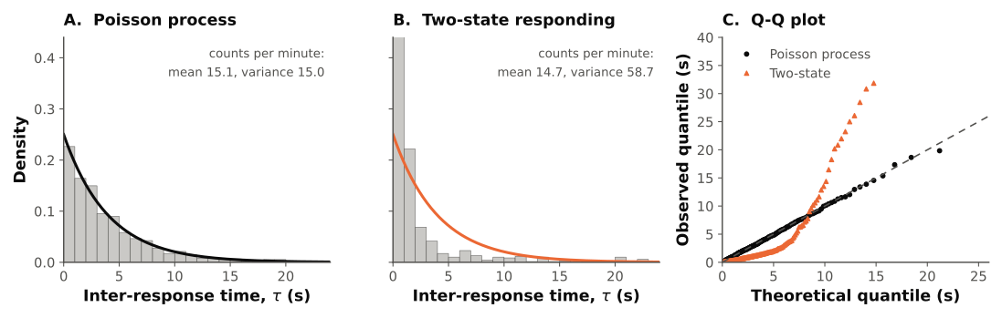
Diagnostics applied to two simulated records with the same response rate

Figure: The three checks above applied to two simulated 50-min records averaging 0.25 responses per second. Both return the same $\hat{\lambda}$ and the same predicted IRT density. Panel A was generated by the Poisson process assuming the observed IRTs track the predicted exponential and the count variance (15.0) matches the count mean (15.1). Panel B was generated by a two-state process (bouts of fast responding separated by long pauses) with the same overall rate. Here, short IRTs are far more common than the exponential predicts, long IRTs are more common as well, and the count variance is roughly four times the mean. The Q-Q plot (C) separates the two records. The Poisson record falls on the diagonal; the two-state record sits below it at short quantiles and climbs steeply above it at long ones, which is the signature of a mixture of rates rather than one constant rate.

Solve:

Given $\hat{\lambda} = 0.25$ resp/s, predict the probability of observing 0 responses in a 10-s interval: $P(0) = e^{-0.25 \times 10} = e^{-2.5} \approx 0.082$ .
Predict the probability that an IRT exceeds 10 s: $P(\tau > 10) = e^{-0.25 \times 10} = e^{-2.5} \approx 0.082$ .
Predict the probability of observing 20 or more responses in a 1-minute bin: compute $P(k \geq 20) = 1 - \sum_{k=0}^{19} P(k)$ using the Poisson distribution with $\lambda t = 15$ . Using standard tables or software, this probability is approximately 0.125. So about 12% of 1-minute bins should contain 20 or more responses if the model is correct.

When to reject the model: If the observed IRT distribution has a mode substantially greater than zero (e.g., a peak at 2-3 seconds rather than near zero), the exponential distribution is inadequate. This pattern often indicates a refractory period (i.e., a minimum time between responses below which the organism cannot or does not respond). If the observed count variance is substantially greater than the mean (overdispersion), the constant-rate assumption is likely violated. If the autocorrelation of successive IRTs is significantly positive, responses are clustered in bursts. Each of these diagnostics points toward a specific kind of model extension, illustrating how probabilistic models fail informatively rather than silently.

Worked Example

This section provides detailed examples of Bayesian updating for a clinical assessment question and maximum likelihood estimation for a Poisson rate parameter. Both examples are worked step by step so that you can follow the calculations and, more importantly, see how the conceptual ideas translate into concrete numbers.

Part 1: Bayesian Updating

Suppose you are evaluating whether a particular consequence (adult attention) is maintaining a child's problem behavior. You want to estimate $p$ , the probability that any given instance of the problem behavior is followed by attention in the natural environment.

Setting up the prior. Before collecting data, you have no strong belief about the value of $p$ . You adopt a uniform prior over the interval [0, 1]:

p(\text{prior}) = \text{Beta}(1, 1).

The Beta(1, 1) distribution is flat (i.e., every value of $p$ between 0 and 1 is equally likely). This reflects maximal uncertainty.

Observing data. You conduct 10 observation intervals. In 8 of the 10 intervals, the problem behavior was followed by attention. In 2 intervals, it was not. So the data are: 8 successes out of 10 trials.

Computing the posterior. The binomial likelihood for $k$ successes in $n$ trials with probability $p$ is:

P(\text{data} | p) = \binom{n}{k} p^k (1-p)^{n-k} = \binom{10}{8} p^8 (1-p)^2.

When the prior is $\text{Beta}(\alpha, \beta)$ and the data are binomial, the posterior is also a Beta distribution (the Beta is the conjugate prior for the binomial):

p(\text{posterior}) = \text{Beta}(\alpha + k, \beta + n - k) = \text{Beta}(1 + 8, 1 + 2) = \text{Beta}(9, 3).

Interpreting the posterior. The Beta(9, 3) distribution has:

Posterior mean: $\frac{9}{9 + 3} = \frac{9}{12} = 0.75$
Posterior mode: $\frac{9 - 1}{9 + 3 - 2} = \frac{8}{10} = 0.80$
95% credible interval: approximately [0.48, 0.94]

Before collecting data, every value of $p$ was equally plausible. After observing 8/10 intervals with attention following behavior, the posterior is concentrated around $p = 0.75$ to $0.80$ , with a 95% credible interval of roughly [0.48, 0.94]. The data have substantially reduced our uncertainty, but a wide range of values remains plausible with only 10 observations.

Updating again. Now suppose you collect 10 more observations and 7 out of 10 show attention following behavior. The posterior from the first batch, Beta(9, 3), becomes the prior for the second batch. The new posterior is:

\text{Beta}(9 + 7, 3 + 3) = \text{Beta}(16, 6).

This distribution has:

Posterior mean: $\frac{16}{22} \approx 0.727$
Posterior mode: $\frac{15}{20} = 0.75$
95% credible interval: approximately [0.52, 0.89]

The credible interval has narrowed. With 20 observations (15 successes), we are more confident that $p$ is in the range of 0.5 to 0.9, with the most likely values around 0.73 to 0.75.

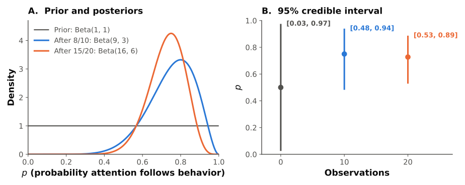
Prior and posterior distributions across two batches of observations

Figure: The two rounds of updating worked in the text.

What this illustrates. Bayesian updating is cumulative with each batch of data. The posterior from one analysis becomes the prior for the next, so evidence accumulates naturally. With a uniform prior, the posterior mean after all data is simply the observed proportion (15/20 = 0.75), which matches the frequentist estimate. The Bayesian framework adds the credible interval, which directly answers the question "what range of values is plausible given the data?"

Note that the order in which data arrive does not matter. Whether you observe 8/10 and then 7/10, or 15/20 all at once, the final posterior is Beta(16, 6). This is a consequence of the mathematics because the product of likelihoods is commutative. It also means that Bayesian updating can be applied in real time (updating after each observation) or in batches (updating after a block of observations) with identical results.

Why this matters for clinical practice. In applied behavior analysis, practitioners routinely collect data across sessions and update their clinical judgment about whether a treatment is working. Bayesian updating provides a formal framework for this process. Instead of relying on visual inspection alone (which is susceptible to bias and inconsistency), a Bayesian analysis provides a quantitative answer: "Given all the data collected so far, the probability that the treatment effect exceeds a clinically meaningful threshold is X%." This does not replace clinical judgment, but it supplements it with a principled quantitative tool.

Part 2: Maximum Likelihood Estimation for a Poisson Rate

A researcher records the number of stereotypic hand movements in successive 1-minute observation intervals. The observed counts are:

Interval	1	2	3	4	5	6	7	8	9	10
Count	3	5	2	4	6	3	4	5	2	4

We assume that the count in each interval is drawn from a Poisson distribution with rate $\lambda$ .

Step 1: Write the log-likelihood. The log-likelihood for Poisson data is:

\ell(\lambda) = \sum_{i=1}^{n} \left[ k_i \ln \lambda - \lambda - \ln(k_i!) \right].

Substituting $n = 10$ and the observed counts:

$\ell(\lambda) = (3 + 5 + 2 + 4 + 6 + 3 + 4 + 5 + 2 + 4) \ln \lambda - 10\lambda - \sum_{i=1}^{10} \ln(k_i!)$ , and

\ell(\lambda) = 38 \ln \lambda - 10\lambda - C,

where $C = \sum \ln(k_i!)$ is a constant that does not depend on $\lambda$ .

Step 2: Find the maximum. Take the derivative with respect to $\lambda$ and set it equal to zero:

\frac{d\ell}{d\lambda} = \frac{38}{\lambda} - 10 = 0,

\hat{\lambda} = \frac{38}{10} = 3.8

Step 3: Verify it is a maximum. The second derivative is:

\frac{d^2\ell}{d\lambda^2} = -\frac{38}{\lambda^2}.

This is negative for all $\lambda > 0$ , confirming that $\hat{\lambda} = 3.8$ is a maximum.

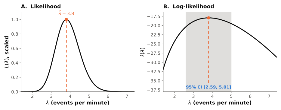
Likelihood and log-likelihood for the Poisson rate

Figure: The likelihood for the ten counts above. Panel A is the likelihood $L(\lambda)$ , scaled so its maximum is 1; Panel B is the log-likelihood $\ell(\lambda)$ . Taking logs turns the product over the ten intervals into a sum and does not move the maximum, which sits at $\hat{\lambda} = 3.8$ in both panels. The curvature of the log-likelihood at its maximum is what the standard error measures. A flatter peak means a wider range of rates account for the data nearly as well and a correspondingly wider 95% confidence interval (shaded, [2.59, 5.01]).

Step 4: Interpret the result. The maximum likelihood estimate of the Poisson rate is 3.8 events per minute. This is the sample mean of the counts. Under the Poisson model, the variance should also equal 3.8. The observed sample variance is:

s^2 = \frac{1}{n-1}\sum_{i=1}^{n}(k_i - \bar{k})^2 = \frac{1}{9}\left[(3-3.8)^2 + (5-3.8)^2 + \cdots + (4-3.8)^2\right].

Computing: the squared deviations are 0.64, 1.44, 3.24, 0.04, 4.84, 0.64, 0.04, 1.44, 3.24, 0.04. The sum is 15.60, so $s^2 = 15.60/9 = 1.73$ .

The observed variance (1.73) is considerably smaller than the Poisson prediction (3.8). This underdispersion suggests that the counts are less variable than a Poisson model predicts. That is, the responses may be more regularly spaced than random. This is a diagnostic check as the model may not be appropriate even though we can compute an MLE. The constant-rate, independent-events assumptions of the Poisson model may be violated.

Standard error of the estimate. For Poisson MLE, the standard error of $\hat{\lambda}$ is:

SE(\hat{\lambda}) = \sqrt{\frac{\hat{\lambda}}{n}} = \sqrt{\frac{3.8}{10}} = \sqrt{0.38} \approx 0.616.

An approximate 95% confidence interval for $\lambda$ is $3.8 \pm 1.96 \times 0.616 = [2.59, 5.01]$ .

Interpreting the full analysis. The MLE tells us that the best-fitting Poisson rate is 3.8 events per minute. The confidence interval tells us that rates between about 2.6 and 5.0 are consistent with the data. But the variance check tells us something the point estimate does not: the data are less variable than the Poisson model predicts. This could mean that the behavior is more regular than a random process would produce (e.g., stereotypic movements occur at semi-regular intervals). This kind of diagnostic insight is a major advantage of probabilistic modeling because the model's failure mode is informative about potential behavioral processes.

Assumptions and Limitations

Every probabilistic model makes assumptions, and these assumptions can be violated in ways that matter.

Poisson process assumptions.

Constant rate: The Poisson process assumes $\lambda$ does not change over time. Within-session changes in motivation, fatigue, satiation, and schedule interactions all violate this assumption. The Poisson process is most appropriate for short time windows during which the rate is approximately constant.
Independence: The Poisson process assumes that the occurrence of one response does not influence the timing of the next. In practice, responses often occur in bursts (positive dependence) or are followed by mandatory pauses (negative dependence). Post-reinforcement pauses, response bursts, and refractory periods all violate independence.
Identically distributed intervals: All inter-response times are drawn from the same distribution. If the rate drifts or if there are distinct behavioral states (responding vs. pausing), this assumption fails.

Bayesian assumptions.

Choice of prior: Bayesian inference requires specifying a prior distribution. Different priors can lead to different posteriors, especially with small samples. While the influence of the prior diminishes with more data, the choice of prior is a modeling decision that should be justified and subjected to sensitivity analysis.
Model specification: Bayesian updating gives the correct posterior given the model. If the model is wrong (e.g., assuming a binomial when the data are overdispersed), the posterior will be wrong regardless of how carefully Bayes' theorem is applied. Bayesian inference does not protect against model misspecification.

Maximum likelihood assumptions.

Correct model: MLE finds the best parameters for the specified model. If the model is wrong, the MLE will faithfully find the best parameters of the wrong model. Goodness-of-fit checks are essential.
Sample size: MLE has desirable properties (consistency, efficiency) in large samples. In small samples, MLE can be biased, and the normal approximation used for confidence intervals may be poor.
Independence: Standard MLE assumes independent observations. Autocorrelated data (common in time-series behavioral data) require modified approaches.

Signal detection assumptions.

Equal-variance Gaussian distributions: The standard $d'$ measure assumes that the signal and noise distributions are both normal with equal variances. If the variances are unequal (which is common), $d'$ can be misleading. More general SDT models allow unequal variances.
Single criterion: The standard model assumes a fixed decision criterion. In practice, observers may shift their criterion within a session based on base rates, payoffs, or fatigue.

General independence assumptions. Many probabilistic models assume that successive observations are independent. In time-series data (i.e., most behavioral data) this assumption is frequently violated. Response rates in consecutive intervals are often positively correlated (if the organism is responding fast in one interval, it tends to respond fast in the next). IRTs may be serially correlated (a short IRT tends to be followed by another short IRT, reflecting response bursts). Ignoring these dependencies does not necessarily bias point estimates, but it can significantly underestimate uncertainty with standard errors becoming too small, confidence intervals too narrow, and significance tests too liberal.

Model misspecification. All of the methods covered this week assume that the model being used is at least approximately correct. If the model is fundamentally wrong the results can be misleading in ways that are not always obvious (e.g., using a Poisson model for data that are actually negative binomial, or using an equal-variance SDT model when variances are unequal). The best defense against model misspecification is to check the model's predictions against the data as we have in past weeks. Examine residuals, compare observed and predicted distributions, and test specific implications of the model's assumptions.

The general lesson. Every probabilistic model makes specific assumptions about the form of randomness (which distribution, which dependence structure, which parameters are constant). These assumptions are testable, and testing them is part of the modeling process. A Poisson model that shows overdispersion is telling you something important about the behavioral process---something a deterministic model would miss entirely. The assumptions are not obstacles to be overcome; they are tools for learning about the phenomenon.

Connection to Empirical Behavior Science

Probabilistic models have a long history in the experimental analysis of behavior, even if they are not always labeled as such.

Inter-response time distributions. The study of IRT distributions has been a staple of operant research since the 1950s. Anger (1956) analyzed IRT distributions on VI schedules and showed that they were approximately exponential, consistent with a Poisson process. Subsequent work revealed systematic departures from the exponential (i.e., short IRTs reflecting response bursts, long IRTs reflecting pauses) that pointed toward more complex models (e.g., mixture distributions with separate "burst" and "pause" components). Shull, Gaynor, and Grimes (2001) proposed a two-state model in which the organism alternates between an "engaged" state (with high response rate) and a "disengaged" state (with zero or near-zero response rate). Within the engaged state, responses follow a Poisson process. The observed IRT distribution is a mixture of short IRTs (from within-bout responding) and long IRTs (from between-bout pauses). This model is a direct extension of the Poisson process framework introduced this week.

VI schedule performance. The variable-interval schedule itself can be modeled as a Poisson process where reinforcement becomes available at random times according to an exponential distribution of inter-reinforcement intervals. The interaction between the Poisson process generating reinforcement availability and the organism's response process creates the characteristic VI performance pattern. Understanding this interaction requires probabilistic modeling.

A key insight from the probabilistic perspective is that on a VI schedule, the obtained reinforcement rate depends on both the programmed rate and the organism's response rate. If the organism stops responding, reinforcers accumulate in the "waiting" state, and the next response has a high probability of contacting reinforcement. If the organism responds very rapidly, most responses are unreinforced because the interval has not yet elapsed. This interaction can be modeled as two stochastic processes (schedule and organism) and generates the curvilinear relationship between programmed and obtained reinforcement rates that Herrnstein's hyperbola describes. The hyperbolic function, introduced in Week 1 as an algebraic model, thus has roots in probability theory.

Conditional probability in contingency analysis. The concept of contingency (i.e., the relationship between behavior and its consequences) is fundamentally a statement about conditional probabilities. The degree of contingency can be defined as the probability of reinforcement given a response, $P(SR|R)$ , versus the probability of reinforcement given no response, $P(SR|\text{no } R)$ . When $P(SR|R) > P(SR|\text{no } R)$ , there is a positive contingency. When they are equal, there is no contingency (a non-contingent or response-independent schedule). Hammond (1980) and others formalized contingency analysis in these probabilistic terms, connecting the language of operant conditioning to the language of probability theory.

Signal detection in observational measurement. Behavioral observation inherently involves signal detection. An observer watching a video must decide, moment by moment, whether the target behavior is occurring. Inter-observer agreement statistics (e.g., Cohen's kappa) are useful but confound sensitivity and bias. SDT provides an alternative analysis, separating the observer's ability to detect the behavior from the observer's threshold for calling it present. This approach has been applied to studies of observer training, coding system design, and measurement reliability.

Bayesian approaches to single-case design. Recent developments in single-case experimental design have adopted Bayesian methods for analyzing phase-change data. Instead of relying on visual analysis alone, Bayesian models can quantify the probability of a treatment effect, accumulate evidence across phases, and incorporate prior information from previous cases or the literature. These approaches are still developing but apply the tools introduced this week.

Stochastic models of reinforcement learning. Modern computational models of learning (e.g., temporal difference learning, Bayesian models of classical conditioning) are fundamentally probabilistic. They model the organism as estimating probabilities and updating estimates in light of experience, much as Bayes' theorem prescribes. The Rescorla-Wagner model, introduced in an earlier week as a deterministic model of associative strength change, can be recast in probabilistic terms where the prediction error on each trial is treated as a noisy estimate of the true discrepancy between expectation and outcome. This probabilistic reinterpretation opens the door to formal model fitting via MLE or Bayesian inference. This connects the learning model to the estimation tools introduced this week.

Statistical process control. In applied settings, statistical process control (SPC) charts are increasingly used to monitor client behavior over time. A control chart plots observed values against expected values (derived from a probability model) and flags observations that fall outside the expected range. A simple version uses the Poisson distribution. If the baseline rate of problem behavior is $\lambda = 5$ per hour, the upper control limit might be set at $\lambda + 3\sqrt{\lambda} = 5 + 3(2.24) = 11.7$ . An observation exceeding this limit is flagged as statistically unusual, prompting investigation. This is a direct, practical application of the Poisson model to clinical decision-making.

Probability in applied behavior analysis. The applied wing of behavior science has been slower to adopt formal probabilistic models, but the tools introduced this week have clear applications. Interval-based behavioral observation is a signal detection task. Treatment evaluation in single-case designs involves reasoning about whether observed changes exceed what would be expected by chance which is a probabilistic question. The growing use of quantitative methods in applied settings (e.g., Bayesian analysis of phase-change data, statistical process control charts for monitoring behavior) reflects the increasing recognition that probabilistic reasoning is not just for basic researchers.

Exercises for Reflection

These exercises are designed to deepen your understanding of the probabilistic tools introduced this week. For each exercise, show your work and explain your reasoning in plain language as well as mathematical notation. The goal is to get the right number as well as demonstrate that you understand what the number means.

A rat on a VI 30-s schedule presses the lever at a steady rate of 20 responses per minute. If you model the presses as a Poisson process, what is the probability of observing exactly 5 presses in a 15-second interval? What is the probability of observing zero presses in a 15-second interval? Show your calculations and interpret the results in the context of the experimental scenario. What would it mean, practically, to observe zero presses in a 15-second window?
You are using Bayesian updating to estimate the probability $p$ that a client engages in problem behavior during a therapy session. Your prior is Beta(2, 2), reflecting a mild belief that $p$ is near 0.5. You observe 3 sessions with problem behavior and 7 sessions without. What is the posterior distribution? What is the posterior mean? How does the result change if you start with a uniform prior, Beta(1, 1), instead? What does this tell you about the influence of the prior with this amount of data?
Two behavioral observers independently code 100 intervals for the presence or absence of self-injurious behavior. Observer A reports behavior in 40 intervals; Observer B reports behavior in 25 intervals. They agree on 20 intervals where behavior was present and 55 intervals where it was absent. Using signal detection theory concepts (not necessarily formal SDT calculations), explain how differences in sensitivity vs. differences in criterion could account for the discrepancy between observers. Why is this distinction important for interpreting inter-observer agreement? If you were training observers to improve agreement, would your training approach differ depending on whether the problem was sensitivity or criterion? Explain.
You fit a Poisson model to response counts and find that the observed variance is three times the observed mean. What does this overdispersion tell you about the assumptions of the Poisson model? Name two behavioral processes that could produce overdispersion and explain the mechanism. What alternative model might you consider? How would you test whether the alternative model provides a better account of the data?

Key Readings

Otto and Day (2007, Primer 3) provided a self-contained introduction to probability theory, covering random variables, expected values, variance, and the key distributions (i.e., binomial, Poisson, normal) that arise most frequently in biological and behavioral data. They also developed conditional probability and Bayes' theorem from first principles, connecting these ideas to the problem of updating beliefs in light of new evidence. Their treatment of the geometric and exponential distributions is the direct mathematical background for the inter-response time material in this week's framework example. This primer builds the mathematical foundation that supports everything else this week. Without a working understanding of probability distributions, it is difficult to meaningfully engage with maximum likelihood estimation, model comparison via likelihood ratios, or the interpretation of stochastic behavioral data.

Otto and Day (2007, Chapter 13) extended that foundation into probabilistic modeling, taking classic deterministic models and rebuilding them so that chance enters explicitly. They worked through stochastic versions of exponential and logistic growth, a continuous-time birth-death process in which events occur at random points in time, and models of allele frequency change, then illustrated the breadth of the approach with models of cancer development, spatial extinction and recolonization, and coalescent theory. Two of their distinctions transfer directly to behavior. The first is between demographic stochasticity, which arises because each individual event is itself chancy, and environmental stochasticity, which arises because the conditions governing those events fluctuate; the behavioral parallel is variability generated by the response process itself versus variability generated by shifting establishing operations and schedule context. The second is their reliance on simulation: once chance is in the model, many questions are easier to answer by generating many realizations than by solving equations. This week's lab takes the same approach. A model that specifies a distribution can be tested against the shape of the data, not only against its mean.

Note that the estimation methods this week uses (likelihood functions, maximum likelihood estimation, confidence intervals) are developed in Otto and Day's Chapters 14 and 15, which are not assigned. Chapter 13 builds the stochastic models. The worked examples in this chapter supply the tools for fitting them.

Reading Guide

Otto & Day (2007): Probability Theory (Primer 3)

What is the difference between a probability and a probability distribution? Why is this distinction important for modeling behavioral data?
How do Otto & Day define a random variable? Give an example of a behavioral measure that would be modeled as a discrete random variable and one that would be modeled as a continuous random variable.
What is the expected value of a random variable, and how does it relate to the concept of a "typical" observation in behavioral data?
What is variance, and why is it important to quantify when modeling behavior? How does variance relate to the precision of our predictions?
What is a Bernoulli trial? Describe a behavioral observation that could be modeled as a Bernoulli trial.
How is the binomial distribution derived from Bernoulli trials? When would you use a binomial model in behavior science?
What conditions must be met for a Poisson distribution to be appropriate? Give a behavioral example where these conditions are approximately satisfied.
What is a probability density function, and how does it differ from the way probability is assigned in a discrete distribution? Why can a density exceed 1 when a probability cannot?
How do Otto & Day describe the normal distribution? Why is the normal distribution so common in statistical applications, even when individual observations are not normally distributed?
Otto & Day derive the geometric distribution as the number of trials until the first success. What behavioral quantity would that describe, and what does its memoryless property imply about responding?
The exponential distribution is the continuous analogue of the geometric. How do Otto & Day relate it to events occurring at a constant rate, and how does that connect to the inter-response time distribution used in this week's framework example?
What is the central limit theorem, and why is it relevant for estimating means from behavioral data?
How do conditional probabilities relate to behavioral contingencies? Can you express a reinforcement contingency as a conditional probability?
What is Bayes' theorem, and how does it update prior beliefs in light of new evidence?
Why do Otto & Day emphasize the importance of understanding probability theory before building probabilistic models?

Otto & Day (2007): Probabilistic Models (Chapter 13)

How do Otto & Day define a stochastic model (Definition 13.1)? How does describing "the probability of a system being in different states" differ from predicting a single state?
What distinguishes a probabilistic model from a deterministic model? When might a probabilistic model be more appropriate for behavioral data?
The authors take deterministic models they had already built and add chance to them rather than starting over. Trace that move for one model in section 13.2. What stays the same, and what has to be specified that the deterministic version never needed?
What is the difference between demographic and environmental stochasticity? Give a behavioral example of each, and explain why the distinction changes what you would do about the variability.
In the birth-death model of section 13.3, events occur at random points in continuous time. How do the authors characterize the waiting time between events, and how does that relate to the Poisson process introduced this week?
What is a transition probability, and what role does it play in describing how a stochastic model moves from one state to the next?
Why do the authors rely so heavily on simulation in this chapter? What kinds of questions about a stochastic model are easier to answer by generating many realizations than by solving equations?
What is an individual-based model (section 13.7), and what does tracking individuals separately provide that tracking an aggregate does not? What would the behavioral analogue be?
The models in this chapter are drawn from ecology and evolution. Pick one (population growth, birth-death, Wright-Fisher, or the cancer model) and describe a behavioral phenomenon with the same stochastic structure. What plays the role of a birth, a death, and the population?
What is a stochastic process, and how might it describe the sequence of responses an organism emits during a session?
Otto & Day note at the end of section 13.1 that methods for analyzing stochastic models come in the following two chapters. Given that, what can this chapter alone tell you about a model, and what does it leave open?
How do the authors suggest balancing mathematical tractability with biological (or behavioral) realism when building probabilistic models?

References

Anger, D. (1956). The dependence of interresponse times upon the relative reinforcement of different interresponse times. Journal of Experimental Psychology, 52(3), 145--161. https://doi.org/10.1037/h0041255

Hammond, L. J. (1980). The effect of contingency upon the appetitive conditioning of free-operant behavior. Journal of the Experimental Analysis of Behavior, 34(3), 297--304. https://doi.org/10.1901/jeab.1980.34-297

Otto, S. P., & Day, T. (2007). A biologist's guide to mathematical modeling in ecology and evolution. Princeton University Press.

Shull, R. L., Gaynor, S. T., & Grimes, J. A. (2001). Response rate viewed as engagement bouts: Effects of relative reinforcement and schedule type. Journal of the Experimental Analysis of Behavior, 75(3), 247--274. https://doi.org/10.1901/jeab.2001.75-247

Key Takeaways

Behavioral data are inherently variable. Probabilistic models treat variability as a feature to be modeled, not noise to be eliminated.
Key distributions for behavior science: The binomial (discrete trials, choice), the Poisson (event counts in time), and the normal (continuous measurements, error).
The Poisson process models events occurring randomly at a constant rate. It predicts Poisson-distributed counts and exponentially distributed inter-event times. It is the simplest model for operant response timing.
Bayes' theorem provides a principled method for updating beliefs in light of new evidence: posterior $\propto$ likelihood $\times$ prior.
Bayesian updating is iterative: each posterior becomes the next prior, so evidence accumulates naturally over successive observations.
Maximum likelihood estimation finds the parameter values that make the observed data most probable. It is the standard method for fitting models and is built on the likelihood function, not the probability function.
Likelihood is not probability. The likelihood function evaluates how well each parameter value accounts for the data; it is not a probability distribution over parameters.
Signal detection theory separates an observer's sensitivity ( $d'$ ) from response bias ( $c$ ), providing a more informative analysis of discrimination and observation than raw agreement or accuracy.
Stochastic models predict distributions, not point values. They are more honest about uncertainty than deterministic models and provide richer diagnostics when assumptions are violated.
Assumption checking is essential. Every probabilistic model assumes a specific form of randomness. Testing those assumptions (e.g., checking for overdispersion, autocorrelation, or normality) is part of responsible modeling practice.
Probabilistic models fail informatively. When a probabilistic model's predictions are violated (e.g., observed variance does not equal predicted variance), the nature of the failure points toward specific model extensions. This is a major advantage over deterministic models, which offer no principled way to characterize the residual variability.
The tools introduced this week underpin everything that follows. Parameter estimation, model comparison, and the interpretation of model fit all rely on probability theory. Mastering these fundamentals is essential for the remaining weeks of the course.