Week 7: How to Construct a Model

Why This Topic Matters

Up to this point, we have focused on understanding, analyzing, and comparing existing models. You have encountered the matching law, discounting functions, demand curves, and associative models. You have learned to identify parameters, check dimensional consistency, and evaluate goodness of fit. All of that work took place on models someone else had already built. This week you get to build the model yourself from the ground up.

The shift from user to builder is the hardest transition in a modeling course but the most important one. Analyzing a finished model is like reading a well-edited essay. You can appreciate its structure, evaluate its arguments, and spot its weaknesses. Building a model is like writing that essay from a blank page. And, staring at a blinking cursor on a blank page is where many people get stuck.

The biggest barrier to model building is rarely the mathematics. Rather, it is the assumption that the model must be correct and complete from the start. It does not. Model building is an iterative process and rarely ends. You start with the simplest representation you can write down, check it against what you know, find where it fails, and revise. The first version of every successful model in science was wrong in important ways. The value of the first version is that it gave the modeler something to criticize and improve.

Otto and Day (2007) formalized this iterative process into a set of explicit steps. Their approach maps closely onto the 8-step framework we have used throughout the course and provides a task analysis for going from a behavioral question to a working mathematical model. This week teaches that sequence of steps.

The practical skills you develop here are the core skills of quantitative behavior science. These include drawing diagrams, translating diagrams into equations, checking units, running sensitivity analyses, and estimating parameters. They are the tools you will use in every subsequent week of the course, and they are the tools you will need if you ever want to build a model of a behavioral phenomenon in your own research.

There is also a theoretical benefit to model building that goes beyond the model itself. The act of mathematically formalizing a behavioral phenomenon forces you to confront what you actually know and what you assume. Can you specify quantitatively the precise functional relationship between reinforcement rate and response rate? Can you say with exactitude what happens to behavior when two contingencies are in effect simultaneously? The model-building process often reveals such gaps in our knowledge and that gap becomes a research question waiting to be asked. Many of the most productive lines of research in quantitative behavior analysis began with someone trying to build a model and discovering that the necessary data did not yet exist or that there were many assumptions that needed to be tested.

Core Concepts

The Iterative Modeling Process

Otto and Day (2007) describe model construction as a cycle with seven steps:

Formulate the question. What do you want the model to do? Predict behavior under new conditions? Explain a known regularity? Identify which processes are necessary and sufficient to produce a phenomenon?
Determine the basic ingredients. What are the essential variables and parameters? What can be measured? What must be estimated?
Qualitative description. Draw a diagram (i.e., a picture) of how the parts of the system interact. This is the most underappreciated step. A good diagram does most of the intellectual work and the math follows from it.
Quantitative description. Translate the diagram into equations. Each arrow in the diagram becomes a term in an equation. Each box or node becomes a variable with its own equation.
Analyze the equations. Find equilibria, check stability, solve for special cases. Determine what the model predicts under different parameter values.
Checks and balances. Verify dimensional consistency. Test limiting cases. Compare predictions to known results. If the model fails these checks, return to an earlier step and revise.
Relate back to the original question. Does the model answer the question you started with? If not, what is missing? What new questions does the model raise?

These steps are cyclic and best thought of as an iterative process. They are not conducted sequentially and a single time. You will often return to Step 1 after reaching Step 6 because the process of building the model clarifies what the real question is. You will revise your diagram after analyzing the equations because the analysis reveals dynamics you did not anticipate. This cycling is not a sign of failure. Iteration is how modeling (and science) works.

The 8-step framework used in this course maps onto Otto and Day's cycle with additional emphasis on stating assumptions explicitly (Step 4 of our framework) and specifying starting values and constraints (Step 7 of our framework). The two systems are complementary, not competing.

An example: Consider a graduate student who wants to model how a child's tantrums change during an extinction procedure. On the first pass, she draws a simple diagram with one variable (tantrum rate) decreasing over time due to extinction. She writes an exponential decay equation, simulates it, and compares it to data. The model captures the overall downward trend but misses the extinction burst. So she returns to Step 3 and adds a process for the extinction burst (perhaps a temporary increase in response variability when reinforcement is first withheld). She redraws the diagram, adds a term to the equation, simulates again. Now the model captures the burst but the timing is off. She adjusts parameters (Step 7), checks units again (Step 6), and iterates. After three or four cycles, she has a model that captures the key features of the data and makes testable predictions about how the burst magnitude depends on the reinforcement history. Each cycle brought the model closer to being useful. Not perfect, but useful. And, once she has a useful model, she can then start comparing how well it generalizes to new data from new experiments and clinical settings.

Life-Cycle Diagrams

A life-cycle diagram is used for discrete-time processes (i.e., systems where events occur in identifiable, sequential stages within each time step). The diagram is drawn as a ring standing for one full cycle. The census, where the variable you are tracking gets counted, sits at the top, and each event that occurs within the cycle is named around the ring in the order it happens. The value of the variable is marked just inside the ring and primed as it passes each event, so you can see what it is worth at every point in the cycle.

Life-cycle diagrams are natural for any process that can be described as "first this happens, then this happens, then this happens, and then the cycle repeats."

Behavior Analytic Example: Lever Pressing Under a Random-Ratio Schedule. Before drawing anything, choose the time scale for a single cycle. Seconds, minutes, and hours are all defensible choices, and that choice determines what "rate of responding" means and what the parameters are measured against.

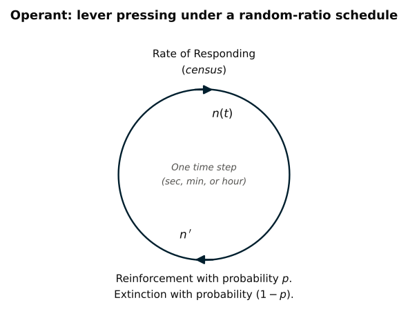
Life-cycle diagram for lever pressing under a random-ratio schedule

Figure: The life-cycle diagram for lever pressing under a random-ratio schedule.

The census at the top counts the current rate of responding, $n_t$ . One event then occurs, in which each response contacts reinforcement with probability $p$ set by the random-ratio schedule. After that event responding stands at $n'$ , and the cycle repeats.

This simple life-cycle diagram is useful, but a question immediately arises as to exactly how $n_t$ is transformed into $n'$ . Assuming only this simple cycle is at play, it seems safe to assume that two processes act on responding within the cycle. First, the increase from reinforcement could be modeled as $\alpha p$ (not the assumption of an interaction). Second, the decrease in responding due to extinction and fatigue can be defined as $\beta$ . Through one cycle, the net change in responding could then be modeled as $n\cdot(\alpha p - \beta)$ .

Now the diagram is starting to show us how it works. By separating the census from the event, it tells us what the recursion has to look like. Something happens to $n_t$ during the cycle, and the result is $n_{t+1}$ . Modeling decisions had to be made on exactly how we transformed $n_t$ to $n_{t+1}$ . But the diagram made this visible rather than letting it slip past.

Now, back to the assumption referenced above. We assumed that reinforcement scales with the behavior already occurring by multiplying our processes by $n_t$ :

n_{t+1} = n_t \cdot \alpha p - \beta n_t.

The assumption here is that the change in response probability is proportional, larger when responding is frequent and smaller when it is sparse.

Alternatively, reinforcement could add a fixed amount per time step:

n_{t+1} = (n_t + \alpha p) - \beta n_t,

so that each reinforcer adds the same amount regardless of how fast the organism happens to be responding.

In both versions $\alpha p$ is the increase from contacting reinforcement and $\beta n_t$ is the decrease from extinction and fatigue.

If forced to choose, we could reach back into the existing behavior analytic literature. Because only so much behavior can occur in a fixed amount of time, the multiplicative version leads toward single-alternative matching and so might be preferred.

Taking the multiplicative version forward, the change across an interval $\Delta t$ is:

\Delta n_t = (\alpha p\,n_t - \beta n_t)\Delta t = (\alpha p - \beta)n_t \Delta t.

This becomes $\frac{dn}{dt} = (\alpha p - \beta) \cdot n_t$ as $\Delta t$ shrinks toward zero, with the solution:

n_t = n_0 \cdot e^{(\alpha p - \beta)t}.

Everything then depends on the sign of $(\alpha p - \beta)$ . If it's positive responding grows exponentially; zero and it holds constant, negative and responding decays exponentially. That single expression now allows us to make precise predictions on how behavior should change over time and becomes the primary benefit for the whole derivation. And, it came out of a diagram carrying two labels.

Behavior Analytic Example: Salivary Responding to a CS. The same construction works on a respondent preparation. Though the two experimental preparations differ significantly, the process of building the model is identical. Here one cycle is one CS presentation.

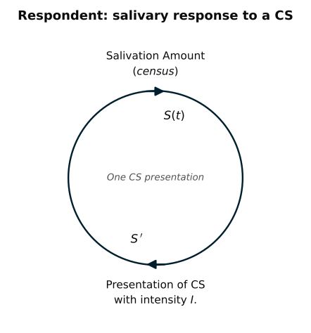
Life-cycle diagram for salivary responding to a conditioned stimulus

Figure: The life-cycle diagram for salivary responding to a conditioned stimulus.

The census records the current salivation level $S_t$ , scaled from 0 to 1. The CS is presented with intensity $I$ , and salivation moves some fraction of the remaining distance toward its asymptotic maximum, leaving $S'$ . The change in salivation could be assumed as proportional to $\gamma I \cdot (1 - S)$ , where $1 - S$ is the remaining distance to maximum association and $\gamma$ is the rate at which the organism learns.

Reading the recursion off the diagram gives the Rescorla-Wagner form:

S_{t+1} = S_t + \gamma I(1 - S_t).

The product $\gamma I$ is the proportion of the remaining distance to asymptote filled in on each trial. A larger $I$ produces a faster approach to asymptote, and as $S_t$ approaches 1 the change per trial shrinks because there is less distance left to cover. Extinction is modeled by reducing $I$ toward zero.

The rest follows as before. The difference equation is:

$\Delta S_t = \gamma I(1 - S_t)\Delta t$ ,

the differential equation is:

$\frac{dS}{dt} = \gamma I(1 - S_t)$ ,

and the solution is:

S_t = 1 - (1 - S_0)e^{-\gamma I t}.

The equilibrium is $S^* = 1$ , and it is always stable as long as $\gamma I > 0$ . The rate of approach is set by $\gamma I$ , so doubling the intensity of the CS doubles the speed of learning. Unlike the operant model above, this one cannot run away, because the $(1 - S_t)$ term shuts growth off as $S_t$ nears its maximum.

Notice that in neither example did we start by inventing an equation and then seeing if it worked. The diagram told us what to track, where the census falls, and what happens in between. Each of those then became a piece of the recursion. The diagram is the blueprint; the equation is the building. Notice also that time advanced in discrete steps in both cases and that, within each step, the system passed through a fixed sequence of events. That is the defining feature of a life-cycle diagram, and it is why the order of events around the ring is a modeling commitment rather than a drawing convenience.

When to use life-cycle diagrams. Life-cycle diagrams are appropriate whenever:

The process unfolds in discrete, identifiable steps (trials, sessions, episodes).
The order of events within a step matters.
The transition from one step to the next depends on what happened during the current step.

Examples from behavior science where life-cycle diagrams might be useful include: discrete-trial instruction, session-by-session changes in performance, trial-based functional analyses, and any procedure with a clear cycle of antecedent-behavior-consequence.

Flow Diagrams

A flow diagram is used for continuous-time processes. That is, systems where quantities change smoothly over time rather than jumping from one stage to another. Each variable, sometimes called a pool or a stock, sits in its own circle labeled with its plain-language name and its symbol. And, every arrow carries a complete rate expression rather than just the parameter name.

Flow diagrams contain four kinds of arrow. An arrow entering a circle from outside is a gain that does not depend on the variable itself. An arrow leaving a circle is a loss. An arrow that loops out of a circle and back into the same circle is the variable generating more of itself, which is the shape that produces exponential growth. And a dashed arrow running into another arrow marks a second variable that the rate of that flow depends on. Together, the set of pools and arrows that comprise a flow diagrams model where one quantity influences another as well as the rate of flow and on what the speed of each flow depends.

Flow diagrams are natural for any process that can be described as "this pool fills up while that pool drains, and the rates depend on the current levels."

Behavior Analytic Example: Concurrent Schedule Behavior Allocation. Consider an organism choosing between two response alternatives (left and right) on a concurrent VI VI schedule. We can think of the organism's behavioral tendency toward each alternative as a "pool" of behavior allocation:

$B_L$ = allocation to the left alternative
$B_R$ = allocation to the right alternative

The flow diagram has two pools. Reinforcement on the left key increases $B_L$ (an inflow). Time without reinforcement on the left key decreases $B_L$ (an outflow due to extinction or decay). The same logic applies to $B_R$ . Additionally, there might be direct competition as increases in rates of responding to $B_L$ necessarily reduce the rate at which responding can occur to $B_R$ . This competiton can be represented as a flow from each pool to the other.

Drawing out the above gives the diagram below.

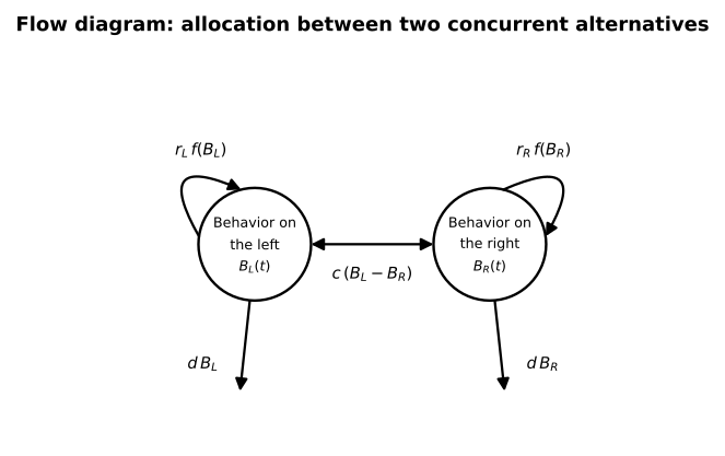
Flow diagram for allocation between two concurrent alternatives

Figure: The flow diagram for concurrent-schedule allocation, drawn in the convention Otto and Day use in Figure 2.4 of the assigned chapter.

Each arrow represents a rate of flow. The reinforcement loops carry rates proportional to the obtained reinforcement rate on each alternative and to how much behavior is already occurring there. This is why they are drawn as loops rather than as arrows arriving from outside. The decay arrows carry rates proportional to the current level of allocation (first-order decay). The reallocation arrow between the two circles carries a sign. The expression $c(B_L - B_R)$ is positive when the responding is higher to the left alternative (i.e., $B_L$ "holds" more behavior) which would shift allocation rightward. And, the reverse occurs when the rate of responding to the right alternative is greater (i.e., $B_R$ "holds" more).

The recipe to translate a flow diagram to a differential equation is:

\frac{dx}{dt} = \sum(\text{rates entering } x) - \sum(\text{rates exiting } x)

This is the fundamental rate flow principle. For the left alternative:

\frac{dB_L}{dt} = r_L \cdot f(B_L) - d \cdot B_L - c \cdot (B_L - B_R),

where $r_L$ is the reinforcement rate on the left, $f(B_L)$ is some function relating current allocation to the effectiveness of reinforcement (e.g., reinforcement schedule), $d$ is the decay rate, and $c$ is a competition parameter. An analogous equation holds for $B_R$ .

The details of $f$ and the specific form of the competition term depend on the theory you are building. The point here is that the flow diagram tells you the structure of the equation. Each arrow contributes a term, inflows are positive, and outflows are negative.

It is worth noticing what this diagram does not give you. In the two life-cycle examples above, one event acted on one variable, and the recursion could be carried all the way to a closed-form solution. Here the two equations are coupled because $B_L$ appears in the equation for $B_R$ and vice versa. So nothing can be solved until you commit to a form for $f$ . What the flow diagram does give you is the equilibrium condition. Setting $\frac{dB_L}{dt} = 0$ gives:

r_L \cdot f(B_L) = d \cdot B_L + c \cdot (B_L - B_R).

This equation says that when allocation stops changing, the inflow from reinforcement exactly balances what decay and reallocation carry away. That is the steady state pattern of choice and it is where a model of this kind makes contact with the matching relations we studied earlier in the course.

When to use flow diagrams. Flow diagrams are appropriate whenever:

The process involves quantities that change continuously (or approximately continuously) over time.
Multiple interacting variables influence each other simultaneously.
You are interested in rates of change, equilibria, and dynamic trajectories.

Examples from behavior science might include: behavior allocation across concurrent schedules, the dynamics of behavioral momentum during disruption, cumulative reinforcement histories, real-time models of response-by-response choice, and any time we want to model when reinforcement rate depends on response rate, which in turn depends on reinforcement rate.

Comparing life-cycle and flow diagrams. The two diagram types are not competing alternatives. Each is a tool best suited to different situations. Sometimes a phenomenon can be modeled either way. Acquisition of a new response, for example, can be modeled as a discrete-time life-cycle process (trial by trial) or as a continuous-time flow process (smooth change in response probability). The choice depends on whether the discrete or continuous representation better matches the data and the question. In practice, many behavior-science phenomena have elements of both. Trials are discrete, but sessions are closely spaced enough that session-to-session change might look continuous (or continuous models prove useful). The modeler must choose a level of description. The diagram type then follows from that choice.

From Diagram to Equation

The most important practical skill in model building is the mechanical translation from diagram to equation. This translation is systematic and, once learned, can prevent errors.

For life-cycle diagrams (discrete time):

Identify the state variable(s) you want to track (e.g., probability of correct responding, number of organisms in a stage).
For each transition arrow that affects the state variable, write a term describing how it changes the variable in one time step.
Sum all terms to get the update rule: $x_{t+1} = x_t + \sum(\text{change terms})$ .

For flow diagrams (continuous time):

Identify each pool (state variable).
For each arrow entering the pool, write a rate expression (positive term).
For each arrow exiting the pool, write a rate expression (negative term).
The derivative equals the sum: $\frac{dx}{dt} = \sum(\text{inflow rates}) - \sum(\text{outflow rates})$ .

The diagram is a visual check on your equation. If you wrote an equation with three terms but your diagram has four arrows, something is missing. If you have a positive term where the diagram shows an outflow, the sign is wrong. The diagram and the equation have to be consistent. If they are not, one of them has an error.

This mechanical process hopefully removes the mystique from mathematical modeling. You do not need to magically create the equation out of thin air. You draw the picture, label the arrows, and build the equation. The intellectual work requiring your domain expertise is in drawing the right picture.

A common mistake is to try to write the equation first without drawing a diagram. This approach works for very simple models but fails quickly as complexity increases. Without a diagram, it is easy to forget a process, double-count a flow, or get a sign wrong. The diagram is a visual accounting system that helps to prevent these errors. Even experienced modelers draw diagrams first because it saves time and prevents mistakes.

Multiple state variables. Many interesting behavioral models (epecially at the boundaries of what we know) involve more than one state variable. When you have two or more pools in a flow diagram, you get a system of equations with one equation per pool. These equations are coupled. That is, the rate of change of one variable depends on the current value of another. For example, in the concurrent schedule model above, $\frac{dB_L}{dt}$ depends on $B_R$ (through the competition term), and $\frac{dB_R}{dt}$ depends on $B_L$ . Coupled systems can produce dynamics that no single equation could generate on its own, including oscillations, stable coexistence, and winner-take-all outcomes.

An example might be useful using a classic predator-prey analog in behavior science. A therapist delivers consequences (the consequence is the "predator") that reduces challenging behavior (the respone repertoire contains the "prey" population), but the therapist's behavior is itself influenced by the level of challenging behavior. When challenging behavior is high, the therapist intervenes more actively; when challenging behavior is low, the therapist may reduce vigilance (e.g., treatment fidelity). This creates a feedback loop:

\frac{dC}{dt} = r_C \cdot C - a \cdot P \cdot T,

\frac{dT}{dt} = b \cdot C \cdot T - d_T \cdot T.

Here, $C$ is rate of challenging behavior, $T$ is therapist intervention intensity, $r_C$ is the baseline rate of increase in challenging behavior, $a$ is the effectiveness of therapist intervention, $b$ is the degree to which challenging behavior evokes therapist intervention, and $d_T$ is the decay rate of therapist vigilance.

This very simple system can produce oscillatory dynamics with cycles of challenging behavior increasing, therapist responding and vigilance then increasing, challenging behavior decreasing, therapist relaxing, and challenging behavior increasing again. Whether such oscillations actually occur in practice is an empirical question, but the model generates the prediction and tells you what to look for in the data assuming you have adequately captured the relevant variables and estimated their paramater values correctly.

Sensitivity Analysis

Once you have a model that is performing well, a common follow-up question is whether the behavior of the system is influenced more by one of the variables compared to others. Sensitivity analysis helps us here. Sensitivity analysis asks, "How does the model's output change when you change a parameter?"

The procedure is straightforward:

Choose a baseline set of parameter values.
Select one parameter to vary.
Systematically change that parameter over a range of values while holding all others constant.
Record how the model's output (the dependent variable of interest) changes.
Repeat for each parameter.

The results tell you which parameters the model is sensitive to (small changes in the parameter produce large changes in output) and which parameter changes the model is robust to (large changes in the parameter produce little change in output).

Sensitivity analysis is important in behavior science for three reasons. First, it identifies the leverage points in a behavioral system. If a model of a token economy is highly sensitive to the exchange ratio but insensitive to the delay between token delivery and exchange, that tells the practitioner where to focus intervention design efforts. Second, it reveals identifiability problems. If two parameters have similar effects on the output, it may be impossible to estimate well both from data (i.e., the model is overparameterized for the available data). Finally, it provides robustness checks. If the model's qualitative predictions change significantly with small parameter perturbations, the predictions are likely not trustworthy.

An example may help. Suppose you have the token economy model from the 8-step walkthrough:

P(t) = P^* + (P_0 - P^*) \cdot e^{-\lambda t}

You want to know which parameter matters most: $\lambda$ (rate of adjustment) or $r_t$ (token economy reinforcement rate, which determines $P^*$ ). Fix baseline values at $P_0 = 20$ , $r_p = 3$ , $r_t = 7$ , $\lambda = 0.3$ . Then:

Vary $\lambda$ from 0.1 to 0.5 while holding everything else fixed. Record $P(10)$ .
Vary $r_t$ from 3 to 11 while holding everything else fixed. Record $P(10)$ .

Compare the range of $P(10)$ values across each sweep. If $P(10)$ changes more when you vary $\lambda$ than when you vary $r_t$ , the model is more sensitive to the rate of adjustment. If the reverse, the model is more sensitive to the intervention intensity. This can then inform clinical practice. Should you focus on making the token economy more influential ( $r_t$ ) or on facilitating faster behavior change ( $\lambda$ , perhaps through prompting or shaping)? Sensitivity analysis can help you answer that with data instead of guessing.

Standard sensitivity analysis has a known limitation in that it varies one parameter at a time. This misses interactions where the effect of changing one parameter depends on the value of another. For example, the effect of increasing $r_t$ might depend on whether $\lambda$ is large or small. More sophisticated methods (e.g., global sensitivity analysis, Latin hypercube sampling) exist but are beyond the scope of this week. For now, one-at-a-time analysis provides a useful first look at model behavior.

Dimensional Analysis

Dimensional analysis is the practice of verifying that every term in an equation has consistent units. It is, arguably, the fastest and most reliable error-detection tool in model building.

The rule is simple. You can only add or subtract quantities with the same units. You can multiply or divide quantities with any units (the result has combined units). Every equation must balance dimensionally.

Example: Consider an update rule for response probability:

p_{t+1} = p_t + \alpha \cdot r_t - \beta \cdot p_t

$p_{t+1}$ and $p_t$ are probabilities (dimensionless, between 0 and 1).
$\alpha \cdot r_t$ must also be dimensionless. If $r_t$ is in reinforcers per minute, then $\alpha$ must have units of minutes per reinforcer. This ensures the product is dimensionless.
$\beta \cdot p_t$ must be dimensionless. Since $p_t$ is dimensionless, $\beta$ must also be dimensionless (or more precisely, have units of per time step, which is absorbed into the discrete-time convention).

If you find yourself adding a rate (responses per minute) to a count (responses), the equation is wrong. If you find a probability exceeding 1 or going below 0, something is wrong with the model's structure or parameter ranges.

Dimensional analysis in practice:

Write the units of every variable and parameter next to the equation.
For each term on the right-hand side, multiply/divide the units.
Verify that every additive term has the same units as the left-hand side.
If any term fails, you have found an error. Fix it before proceeding.

This step typically takes only a few minutes and catches errors that would otherwise take hours to debug computationally.

Common dimensional analysis mistakes in behavioral models:

Confusing rates and counts. Response rate (responses/min) and total responses (count) have different units. An equation that predicts response rate cannot have a term that is a raw count without a time conversion.
Forgetting the time step in discrete models. In a difference equation like $n_{t+1} = n_t + \text{(something)}$ , the "something" must have the same units as $n$ . If $n$ is a count and the "something" involves a rate, you need a $\Delta t$ factor to convert.
Dimensionless parameters that are not. Sometimes a parameter appears dimensionless but actually carries hidden units. For example, a "learning rate" parameter $\alpha$ in a trial-by-trial model implicitly has units of "per trial." Making these units explicit prevents errors when converting between trial-level and time-level models.
Probabilities and proportions. These are dimensionless by definition. Any term added to a probability must also be dimensionless. If your model has $p_{t+1} = p_t + r_t$ where $r_t$ is a rate in reinforcers/min, the equation is dimensionally incorrect and you need a scaling factor to make $r_t$ dimensionless.

Dimensional analysis as a thinking tool. Beyond catching errors, dimensional analysis can actually help you build models. If you know what units the left-hand side has, and you know the units of the quantities available on the right-hand side, dimensional analysis constrains how those quantities can be combined. This is especially useful when you are uncertain about the functional form of a relationship. The units tell you which combinations of variables are possible.

Applying the 8-Step Framework

This section applies the full 8-step framework to construct a model from scratch. The goal is to model the effect of a token economy on problem behavior in a clinical setting.

Step 1: Identify All Environmental and Behavioral Components of the Phenomenon A child in a classroom engages in disruptive behavior (e.g., calling out, leaving seat). The teacher implements a token economy where the child earns tokens for periods without disruptive behavior (i.e., differential reinforcement of other behavior) and exchanges tokens for preferred activities at the end of the day. Over days, the rate of problem behavior decreases. We want to model this decrease quantitatively.

Before proceeding, we need to specify what we mean by "disruptive behavior" and how it is measured. For this model, disruptive behavior is operationally defined as any instance of calling out without raising a hand or leaving the assigned seat without first attaining permission. The measurement is a daily frequency count of the total number of instances recorded during the school day.

We observe the following pattern: problem behavior starts at a high rate (roughly 15-25 instances per day during baseline), decreases rapidly in the first few days of the intervention, and then decreases more slowly, eventually reaching a low but nonzero steady state (roughly 3-8 instances per day). The rate of decrease depends on how many tokens are earned and how preferred the backup reinforcers are. The nonzero steady state is notable. The token economy reduces problem behavior substantially but does not eliminate it entirely.

Step 2: Define the Behavioral Principles, Processes, and Intended Scope of the Model We model the daily rate of problem behavior as a function of the token economy parameters. We do not model within-day dynamics, the specific topography of problem behavior, or social interactions with peers. The model covers a single child, a single response class (disruptive behavior), and a single intervention (token economy with DRO).

The key processes are:

Problem behavior produces some amount of maintaining reinforcement (e.g., attention, escape).
The token economy provides an alternative source of reinforcement contingent on the absence of problem behavior.
Over days, the relative value of the token economy reinforcement versus reinforcement for disruptive behavior shifts behavioral allocation away from problem behavior.

Step 3: Write Down the Behavioral Principles, Known Quantitative Laws, and Functional Relationships

Reinforcement: Behavior is maintained by its consequences.
Behavior allocation: The matching law suggests that the behavior allocated to an alternative is a function of the relative reinforcement obtained from that alternative.
Behavioral momentum / resistance to change: Behavior with a longer reinforcement history is more resistant to disruption, so the initial rate of change may depend on the history.

We will use a simple reallocation model rather than the full matching law, keeping the model tractable. Note the deliberate choice here. The matching law is a more complete framework, but it requires specifying multiple concurrent response alternatives and their reinforcement rates. For a first model, we simplify to a single target behavior and its trajectory over time. If this simple model fails to capture the data, the matching law provides a natural direction for elaboration.

Step 4: State All Simplifying Assumptions Explicitly This step is crucial. Every assumption you state is a potential point of model failure and, therefore, a potential direction for improvement. Being explicit about assumptions is what separates principled modeling from ad hoc curve fitting.

Problem behavior is maintained by a single source of reinforcement at a constant rate $r_p$ (reinforcers per day from baseline contingencies).
The token economy provides reinforcement at rate $r_t$ (token-mediated reinforcers per day), which is constant once the intervention is in place.
Total behavioral output is constant: any decrease in problem behavior corresponds to an increase in appropriate behavior.
The rate of change in problem behavior is proportional to the difference between current allocation and the allocation predicted by the reinforcement ratio.
Day-to-day changes are smooth enough to model with a continuous-time approximation.
The child's motivation for the backup reinforcers does not change over the course of the intervention (no satiation to the token economy reinforcers).
Implementation fidelity is perfect: the teacher delivers tokens consistently according to the schedule.

Each of these assumptions is, strictly speaking, wrong. Baseline reinforcement rates fluctuate. Token economy effectiveness varies. Motivation changes. Implementation is imperfect. But the model must start somewhere, and each assumption can be relaxed in future iterations if the data demand it.

Step 5: Write the Model Verbally, Then Express It Mathematically Verbally: Problem behavior decreases over days at a rate proportional to how far the current rate is from the equilibrium rate predicted by the reinforcement contingencies. The equilibrium rate is determined by the ratio of baseline reinforcement for problem behavior to the total reinforcement available (baseline plus token economy).

Drawing the flow diagram:

There is one pool: $P$ , the rate of problem behavior. There is one inflow (baseline reinforcement maintaining problem behavior) and one outflow (the token economy drawing behavior away from problem behavior toward appropriate behavior).

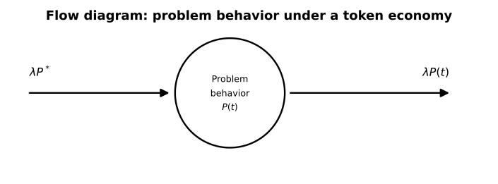
Flow diagram for problem behavior under a token economy

The inflow rate drives $P$ toward the level sustained by baseline reinforcement alone. The outflow rate drives $P$ toward a lower level by providing competing reinforcement.

Mathematically: We can use a first-order approach-to-equilibrium model:

\frac{dP}{dt} = -\lambda \cdot (P - P^*),

where:

$P$ is the current rate of problem behavior (responses per day)
$P^*$ is the equilibrium rate of problem behavior under the token economy (i.e., what matching would predict)
$\lambda$ is the rate constant governing how quickly behavior adjusts (per day)
$t$ is time in days

The equilibrium $P^*$ is determined by the reinforcement contingencies:

P^* = P_0 \cdot \frac{r_p}{r_p + r_t},

where $P_0$ is the baseline rate of problem behavior (before the token economy), $r_p$ is the rate of baseline reinforcement for problem behavior, and $r_t$ is the effective rate of reinforcement from the token economy.

The solution to this differential equation is:

P(t) = P^* + (P_0 - P^*) \cdot e^{-\lambda t}

This is exponential decay from $P_0$ to $P^*$ .

Step 6: Verify Dimensional Consistency

$P$ is in responses per day.
$P^*$ is in responses per day (same units as $P$ so correct).
$P_0$ is in responses per day.
$\lambda$ is in per day (day $^{-1}$ ).
$t$ is in days.
$\lambda \cdot t$ is dimensionless (day $^{-1} \times$ day) so correct for an exponent.
$\frac{r_p}{r_p + r_t}$ is dimensionless (reinforcers per day divided by reinforcers per day) so correct.
$(P_0 - P^*) \cdot e^{-\lambda t}$ is in responses per day so matches $P$ .

All terms are dimensionally consistent.

Step 7: Specify Starting Values and Constraints

$P_0 > 0$ (there must be a baseline rate of problem behavior for the intervention to be meaningful).
$P^* \geq 0$ (the equilibrium rate cannot be negative). Since $P^* = P_0 \cdot \frac{r_p}{r_p + r_t}$ and all rates are non-negative, this is guaranteed.
$\lambda > 0$ (behavior must actually change over time for the model to apply).
$r_p > 0$ (if there is no maintaining reinforcement, there is no problem behavior to model).
$r_t \geq 0$ ( $r_t = 0$ means no intervention, in which case $P^* = P_0$ and nothing changes).

At $t = 0$ , $P(0) = P^* + (P_0 - P^*) \cdot e^0 = P_0$ . This is correct: at the start, problem behavior is at baseline.

As $t \to \infty$ , $P(t) \to P^*$ .

This is correct: the model predicts that problem behavior asymptotes at the level determined by the reinforcement ratio.

Step 8: Check the Math, Test Against Data, and Derive Predictions Verify limiting cases:

If $r_t = 0$ (no token economy), $P^* = P_0$ and $P(t) = P_0$ for all $t$ . The model predicts no change without intervention. Correct.
If $r_t \to \infty$ (extremely powerful token economy), $P^* \to 0$ and the model predicts problem behavior drops to zero. This is an idealization, impossible realistically, but qualitatively correct.
If $\lambda$ is very large, the transition is rapid; if $\lambda$ is very small, it is slow. Both make behavioral sense.

Derive a prediction: Suppose $P_0 = 20$ responses/day, $r_p = 3$ reinforcers/day, $r_t = 7$ reinforcers/day, and $\lambda = 0.3$ per day. Then:

P^* = 20 \cdot \frac{3}{3 + 7} = 20 \cdot 0.3 = 6 \text{ responses/day}

P(t) = 6 + (20 - 6) \cdot e^{-0.3t} = 6 + 14 \cdot e^{-0.3t}

At $t = 5$ days: $P(5) = 6 + 14 \cdot e^{-1.5} = 6 + 14 \cdot 0.223 = 6 + 3.12 = 9.12$ responses/day.

At $t = 10$ days: $P(10) = 6 + 14 \cdot e^{-3.0} = 6 + 14 \cdot 0.050 = 6 + 0.70 = 6.70$ responses/day.

The model predicts that problem behavior drops from 20 to about 9 in the first 5 days, then more slowly approaches 6 over the next 5 days. This negatively accelerated pattern matches what is commonly observed in practice.

Test against data: To validate, collect daily rates of problem behavior during a token economy intervention. Fit the model using nonlinear least squares to estimate $\lambda$ and $P^*$ (or equivalently, $r_p$ and $r_t$ if those are not directly observable). Compare the fitted curve to the data. Assess residuals for systematic deviations.

Iterate: Suppose the residuals show that problem behavior decreases faster than predicted in the first few days but slower than predicted later. This systematic deviation suggests that the constant- $\lambda$ assumption is wrong. For example, perhaps the rate of adjustment itself changes over time (e.g., initial novelty effects wear off). This observation sends us back to Steps 2-4 to revise the model (e.g., make $\lambda$ a decreasing function of time such as $\lambda(t) = \frac{\lambda_0}{1 + kt}$ ). The cycle continues until the model captures the essential features of the data or until we run out of data to constrain additional parameters.

Lessons from this walkthrough. Several features of this example are worth highlighting:

The flow diagram was simple. There was one pool and two arrows. Yet it produced a model with clear, testable predictions.
The dimensional analysis was quick and confirmed the equation was internally consistent.
The limiting-case analysis (Step 8) provided immediate sanity checks without any data fitting.
The numerical predictions ( $P(5) \approx 9.12$ , $P(10) \approx 6.70$ ) give concrete expectations that can be compared to observations.
The model's simplicity also reveals its limitations, pointing toward specific refinements rather than vague dissatisfaction.

Worked Example

Response Acquisition Under Continuous Reinforcement

We will build a model of how a new operant response is acquired when every response produces reinforcement (continuous reinforcement, CRF).

The phenomenon: A rat is placed in an operant chamber. At first, it rarely presses the lever. Each press produces a food pellet. Over time, the rate of lever pressing increases, eventually reaching a stable level. The acquisition curve typically shows an S-shape: slow initial responding (the organism has not yet contacted the reinforcement contingency), followed by a rapid increase (each reinforced response increases the probability of emitting a similar response in the currnte context, which leads to more reinforced responses), followed by a leveling off due to physical or motivational constraints which imposes a ceiling.

We want a model that captures at least the initial accelerating phase of acquisition. A more complete model would also capture the deceleration and asymptote, which we address below.

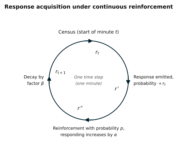
Life-cycle diagram. Within each time step (say, one minute), the following events occur:

The organism begins with a low, but non-zero probability of pressing the lever.
The two response options we track are (a) to press the lever or (b) to not. The probability of pressing the lever is proportional to $r_t$ .
If the organism presses the lever, reinforcement is delivered with probability $p$ (under CRF, $p = 1$ ).
Reinforcement increases the probability of responding for the next time step by a factor $\alpha$ .
Simultaneously, response probability decays by a factor $\beta$ due to fatigue or competing behaviors.

The cycle repeats at the next time step.

Life-cycle diagram for response acquisition under continuous reinforcement

Let's translate the life-cycle diagram to a difference equation. The diagram tells us that response probability increases due to reinforcement and decreases due to fatigue or response competition:

r_{t+1} = r_t + \alpha \cdot p \cdot r_t - \beta \cdot r_t

This can be simplified:

r_{t+1} = r_t \cdot (1 + \alpha \cdot p - \beta)

where:

$r_t$ is the response probability at time step $t$ (arbitrary units, $r_0 > 0$ )
$\alpha$ is the reinforcement effect parameter (dimensionless, $\alpha > 0$ )
$p$ is the probability of reinforcement given a response ( $0 \leq p \leq 1$ ; under CRF, $p = 1$ )
$\beta$ is the response probability decay parameter (dimensionless, $0 < \beta < 1$ )

Dimensional check. All terms are in the same arbitrary units as $r_t$ . The quantities $\alpha \cdot p$ and $\beta$ are dimensionless. The product $r_t \cdot (1 + \alpha \cdot p - \beta)$ has the same units as $r_t$ . Consistent.

Behavior of the model. Define the growth factor $G = 1 + \alpha \cdot p - \beta$ .

If $G > 1$ (i.e., $\alpha \cdot p > \beta$ ), the response probability grows geometrically. Reinforcement effect exceeds decay, and the rate of responding curve is an acquisition curve.
If $G = 1$ (i.e., $\alpha \cdot p = \beta$ ), the response probability is stable. The influence of reinforcement on response probability exactly balances decay.
If $G < 1$ (i.e., $\alpha \cdot p < \beta$ ), the response probability decays. Decay exceeds reinforcement, and the rate of responding is a reduction curve.

This simple model captures geometric growth but has currently no ceiling. As a result, $r_t$ would increase without bound if $G > 1$ . A more realistic model would include an asymptote. For now, we keep it simple and note this limitation. But, we come back to it in a bit.

Simulation with specific parameter values. Let $r_0 = 1$ (initial response probability), $\alpha = 0.15$ (reinforcement effect), $p = 1.0$ (CRF), $\beta = 0.05$ (decay rate).

Then $G = 1 + 0.15 \cdot 1.0 - 0.05 = 1.10$ .

Time step ( $t$ )	$r_t$
0	1.000
1	1.100
2	1.210
3	1.331
4	1.464
5	1.611
6	1.772
7	1.949
8	2.144
9	2.358
10	2.594
11	2.853
12	3.138
13	3.452
14	3.797
15	4.177
16	4.595
17	5.054
18	5.560
19	6.116
20	6.727

The response probability grows geometrically, roughly doubling every 7-8 time steps. Under CRF with these parameters, the model predicts accelerating acquisition. This acceleration is a direct consequence of the multiplicative structure of the model. In each time step, response probability is multiplied by $G = 1.10$ , so the absolute increase per step grows as $r_t$ grows. In the first step, the increase is $0.1 \times 1.0 = 0.1$ . By step 20, the increase is $0.1 \times 6.116 = 0.612$ . This compounding is characteristic of a positive feedback system. More responding leads to more reinforcement, which leads to yet more responding.

The state variable $r_t$ represents response probability, not response rate directly. To connect the model to observable data, we would need a mapping from $r_t$ to actual response rate. For example, response rate could be proportional to $r_t$ , or could be a saturating function of $r_t$ . This mapping is itself a modeling decision that would need to be specified and justified.

Sensitivity analysis: Varying $\alpha$ . We now examine how the model's output at $t = 20$ changes as we vary $\alpha$ while holding $p = 1.0$ , $\beta = 0.05$ , and $r_0 = 1$ constant.

$\alpha$	$G = 1 + \alpha - 0.05$	$r_{20} = G^{20}$
0.05	1.00	1.000
0.08	1.03	1.806
0.10	1.05	2.653
0.12	1.07	3.870
0.15	1.10	6.727
0.20	1.15	16.367
0.25	1.20	38.338

The model is highly sensitive to $\alpha$ . A change from $\alpha = 0.10$ to $\alpha = 0.20$ doubles the reinforcement effect and produces more than a six-fold increase in the response probability at $t = 20$ . This sensitivity makes sense. In a geometric growth model, small changes in the growth rate compound over time.

This sensitivity analysis tells us that if we want to predict acquisition accurately, we need a precise estimate of $\alpha$ . It also tells us that from a practical standpoint, interventions that increase the effectiveness of reinforcement (e.g., using more preferred reinforcers, reducing delay to reinforcement) can have outsized effects on acquisition speed (assuming the model is correct and complete enough to be useful).

The table above also reveals an important property of systems with geometric growth. Specifically, they are disproportionately sensitive to parameters that affect the growth rate. A 100% increase in $\alpha$ (from 0.10 to 0.20) produces more than a 500% increase in $r_{20}$ . This is because each increment to $\alpha$ compounds across all 20 time steps. In practical terms, this would mean that even small improvements in reinforcement effectiveness can significantly accelerate learning. It also means that small decrements can significantly slow it. This is a result that would be difficult to derive from verbal reasoning alone but is readily observable from the model. All of this, again, assuming the model is correct and complete enough to be useful.

As noted above, the geometric growth model has a significant limitation. It has no mechanism for satiation, competing responses, schedule thinning, or motoric constraints. It predicts that response tendency grows without bound as long as $G > 1$ , which is clearly unrealistic. How might we modify our model to handle this?

Adding a ceiling. To prevent unbounded growth, we can introduce a response capacity $K$ :

r_{t+1} = r_t + \alpha \cdot p \cdot r_t \cdot \left(1 - \frac{r_t}{K}\right) - \beta \cdot r_t

This is a logistic-growth analog commonly used in behavioral ecology where environmental carrying capacities limit the growth of populations. When $r_t$ is small relative to $K$ , the model behaves like the original. As $r_t$ approaches $K$ , the reinforcement effect diminishes (a form of saturation or ceiling effect). This extension produces the S-shaped acquisition curve commonly observed in learning data where we observe small initial changes in behavior, rapid behavior change during middle phases, and gradual leveling off.

Simulating the logistic version. With $r_0 = 1$ , $\alpha = 0.15$ , $p = 1.0$ , $\beta = 0.05$ , and $K = 10$ :

Time step ( $t$ )	$r_t$ (geometric)	$r_t$ (logistic, $K = 10$ )
0	1.000	1.000
5	1.611	1.485
10	2.594	2.123
15	4.177	2.890
20	6.727	3.718
25	10.835	4.510
30	17.449	5.181

Note how the logistic model levels off instead of growing without bound. The logistic model is more realistic for most behavioral applications because there are natural ceilings on response rate imposed by physical constraints, competing behaviors, and satiation.

It is worth being precise about where it levels off, because technically it is not at $K$ . Setting $r_{t+1} = r_t$ in the equation above and solving gives:

r^* = K\left(1 - \frac{\beta}{\alpha \cdot p}\right) = 10\left(1 - \frac{0.05}{0.15}\right) = 6.67

Decay never switches off, so responding stops increasing where the influence of reinforcement has been reduced enough to balance decay. The capacity $K$ sets the maximum, but the ratio $\beta / \alpha p$ determines how close to that asymptote responding gets. Raising $\alpha$ or lowering $\beta$ moves the asymptote closer to $K$ without changing $K$ . Note how this offers another testable prediction about what should happen when reinforcer quality improves or effort decreases.

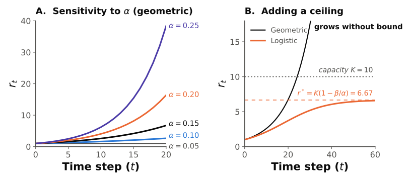
Sensitivity to alpha and the effect of adding a ceiling

Figure: Panel A is the sensitivity analysis from the table above, drawn as trajectories rather than endpoints. Panel B contrasts the two versions at $\alpha = 0.15$ . The geometric model leaves the plot entirely, since nothing in it prevents unbounded growth. The logistic version traces the S-shape seen in real acquisition data and settles at $r^* = K(1 - \beta/\alpha) = 6.67$ . Note that the ceiling the model actually approaches is not the capacity $K$ itself, but $K$ reduced by the ratio of the decay rate to the reinforcement rate. Decay is still removing responding at the asymptote, so growth stops short of capacity.

Connecting the worked example to the framework. This worked example illustrates several principles:

Start simple (the geometric model), then add complexity (the logistic extension). The geometric model was clearly unrealistic (unbounded growth), but it was useful as a starting point because its behavior was easy to understand and it revealed exactly what was missing.
The sensitivity analysis guided our understanding. We learned that $\alpha$ is the critical parameter which holds for the geometric and logistic versions.
The diagram drove the equation. The life-cycle diagram told us which terms to include. Adding the response capacity was a modification of one term, not a complete rewrite.
Dimensional consistency was maintained throughout. Every extension was checked for units before simulation.

Assumptions and Limitations

All models are simplifications and, therefore, require simplifying assumptions. It is important to understand what assumptions you have to make at each stage of model building so that you understand the limitations of your model based on the aproach you have chosen to build a model.

There are several limitations that arise from the assumptions of life-cycle diagrams. First, a life-cycle diagram assumes that events follow a fixed sequence within each time step. If the actual process involves variable ordering or simultaneous events, the diagram may impose false structure and lead to inaccurate predictions. Second, a flow diagram assumes that the pools and flows capture the essential dynamics. If the real system has important discrete events then a continuous-flow model may miss them (e.g., schedule transitions, session boundaries). Lastly, life-cycle and flow diagrams force you to decide which variables are state variables and which are parameters. Your decisions here might be wrong. What you treated as a constant parameter might actually vary in ways that matter.

There are also several limitations to sensitivity analysis. One-at-a-time sensitivity analysis misses interactions between parameters. Using our example above, the effect of changing $\alpha$ might depend on the value of $\beta$ , but varying them independently may not reveal this interaction. Sensitivity analysis also explores the model's behavior, not reality. High sensitivity to a parameter in the model does not mean the real system is sensitive to the corresponding real-world quantity.

Though mentioned in previous weeks, it's worth reiterating that parameter estimation has known limitations. A good fit does not validate a model. Multiple different models (with different assumptions and mechanisms) can fit the same data equally well. Relatedly, parameter estimates are only as good as the data. If the data do not span a wide enough range of conditions, parameters are might be poorly identified.

Connection to Behavior Science

Behavior analysts have, arguably, always been process thinkers. Functional analysis asks what antecedents and consequences maintain behavior? This is, in essence, drawing a flow diagram. The behavior analyst identifies the inputs to and outputs from a behavioral pattern. The step from informal functional process thinking to formal functional model construction is smaller than most behavior analysts realize. If you can describe a three-term or four-term contingency, you can draw a flow diagram. If you can draw a flow diagram, you can write a differential equation.

Consider a standard functional analysis for automatically reinforced self-injurious behavior (SIB). The verbal hypothesis might be that "SIB is maintained by automatic reinforcement (i.e., it produces sensory stimulation that functions as a reinforcer)." A flow diagram version would show a single pool (SIB rate) with an inflow (automatic reinforcement, proportional to the current SIB rate) and an outflow (fatigue, satiation, or competing behaviors). This gives:

\frac{d(\text{SIB})}{dt} = a \cdot \text{SIB} - b \cdot \text{SIB} = (a - b) \cdot \text{SIB}.

Here, $a$ is the automatic reinforcement rate and $b$ is the decay rate. If $a > b$ , the rate of SIB increases; if $a < b$ , the rate of SIB decreases; if $a = b$ , the rate of SIB is stable. This is exactly the kind of analysis that the flow diagram makes transparent. The verbal hypothesis tells you the direction; the formal model tells you the magnitude and trajectory. And, if I know magnitude and trajectory, I can start predicting future behavior.

Otto and Day's (2007) textbook on biodynamics provides one of the most straightforward recipes to translate biological process diagrams into mathematical models. Their life-cycle and flow diagram methods were developed for population biology, but the same methods apply directly to behavioral processes. A population of responses growing and changing through contact with reinforcement is formally analogous to a population of organisms growing and changing through contact with food resources, predation, and sexual interaction. The mathematics of growth, decay, competition, and equilibrium are the same.

The analogy is more than superficial. In population biology, organisms reproduce, compete for resources, and die. In behavior science, responses are emitted, reinforced (selected), and extinguished. The mathematical tools that population biologists use to model selection (i.e., growth equations, competition equations, fitness landscapes) are available to behavior scientists to model reinforcement, competition between response classes, and the evolution of behavioral repertoires. Otto and Day (2007) provide a bridge between these fields, and this week's methods use that bridge.

To close, it might be useful to make explicit the fact that not every model-building effort succeeds. That is acceptable and useful. A model that fails to fit the data is informative. The pattern of failure (which conditions does the model get right? which does it get wrong?) helps the modeler identify which processes are missing or misspecified. In the history of behavior science, some of the most important insights have come from model failures. For example, the failure of simple matching to account for concurrent-chain performance led to the development of delay-reduction theory. And, the failure of exponential discounting to account for preference reversals led to the adoption of hyperbolic discounting. Building models gives you a systematic way to fail productively.

Exercises for Reflection

Choose a behavioral phenomenon from your own research or clinical experience. Draw a flow diagram showing the key variables and the flows between them. Then translate the diagram into a differential equation using the recipe: $\frac{dx}{dt} = \sum(\text{inflows}) - \sum(\text{outflows})$ . Check the dimensional consistency of your equation.
The token economy model in the 8-step walkthrough assumes that the reinforcement rate $r_p$ is constant. In practice, $r_p$ might change (e.g., peers stop attending to problem behavior over time). How would you modify the model to account for a declining $r_p$ ? Write the modified equation and describe qualitatively how the model's predictions would change.
Run a sensitivity analysis (by hand or with a calculator) on the response acquisition model from the worked example. Instead of varying $\alpha$ , vary $\beta$ from 0.01 to 0.20 while holding $\alpha = 0.15$ and $p = 1.0$ . How does $n_{20}$ change? Is the model more sensitive to $\alpha$ or to $\beta$ ? What does this tell you about the relative importance of reinforcement effectiveness versus decay/extinction?
The Euler method approximates continuous change with discrete steps. Using the behavior allocation model $\frac{dB}{dt} = r - d \cdot B$ with $r = 5$ , $d = 0.1$ , and $B_0 = 0$ , compute $B$ at $t = 5$ using (a) $\Delta t = 1.0$ (5 steps), (b) $\Delta t = 0.5$ (10 steps), and (c) the exact solution $B(t) = \frac{r}{d}(1 - e^{-dt})$ . How close is each Euler approximation to the exact solution? What does this tell you about the importance of step size?
Consider a DRA (differential reinforcement of alternative behavior) procedure in which a behavior technician reinforces an alternative communicative response while problem behavior contacts extinction. Draw a flow diagram with two pools: problem behavior ( $P$ ) and alternative behavior ( $A$ ). Include inflows (reinforcement for $A$ , natural reinforcement for $P$ ), outflows (extinction/decay for each), and competition between the pools. Translate your diagram into a system of two differential equations. What does the model predict about the steady-state ratio of $A$ to $P$ ?

Key Readings

Otto and Day (2007, Chapter 2) presented a systematic recipe for constructing mathematical models from scratch, organized as a sequence of steps: formulate the question, identify the variables, draw a diagram, write the equations, and analyze the result. They emphasized that model building is iterative; the first version will be wrong and the value comes from having something concrete to criticize and improve. For this week, the chapter provides the scaffolding that transforms the 8-step framework from an abstract checklist into a practical workflow. The life-cycle and flow diagrams they introduce are especially important, because they make the intellectual work of model construction visual and explicit before any equations are written.

Otto and Day (2007, Chapters 5-6) covered numerical and graphical techniques for understanding model behavior when analytical solutions are unavailable or uninformative. They introduced Euler's method for numerically solving differential equations, phase-plane diagrams for visualizing two-variable systems, nullclines for locating equilibria, and sensitivity analysis for determining how model outputs depend on parameter values. These techniques are the practical tools of model building. And, they allow the modeler to develop intuition about what a model predicts, identify parameter regions where behavior changes qualitatively, and detect unrealistic predictions before investing in formal analysis. For the course, this chapter completes the transition from model consumer to model constructor by equipping you with the computational skills to explore your own models.

Reading Guide

Otto & Day (2007): How to Construct a Model

What is the primary hurdle most new modelers face, and what first step do Otto & Day suggest to overcome it?
The authors introduce seven steps for model construction (Box 2.1). List these seven steps. Why might it be helpful to treat them as iterative rather than strictly sequential?
According to the authors, how does modeling start conceptually, even before equations are written down? What's the benefit of beginning with toy examples?
What distinguishes a dynamical model from other types of models in biology? Give one example of a behavior-analytic phenomenon that would benefit from a dynamical modeling approach.
Explain the difference between deterministic and stochastic models. Why might deterministic models be more appropriate for the current course and lab work?
What makes Step 1---formulating a good question---so difficult for many students? How do Otto & Day suggest you find a starting point?
What are some strategies for simplifying reality when choosing model variables? Why is simplification critical at early stages of modeling?
How can notational conventions like $n(t)$ help prevent errors in reasoning when working with models?
When deciding between a discrete-time and continuous-time model, what key conceptual and behavioral tradeoffs should you consider?
Why do modelers often treat inherently discrete quantities (e.g., number of individuals) as continuous variables? When might this abstraction break down?
Explain the difference between a recursion equation, a difference equation, and a differential equation. What kind of model uses each?
What is the purpose of identifying constraints on variables and parameters during model construction?
Why is it useful to build a table of all variables and parameters before writing your model equations?
Describe the difference between a life-cycle diagram and a flow diagram. When is each most useful?
Describe a situation in behavior analysis where a "life-cycle diagram" might be useful. Do the same for a "flow diagram."
Why is the order of events especially important in discrete-time models?
What does it mean to say a model "fails to capture the essence of the biological process"?
What is the process for turning a flow diagram into equations for a continuous-time model?
How do you know when your model is "done"?

Otto & Day (2007): Numerical and Graphical Techniques

What are the two broad reasons Otto & Day give for using numerical techniques instead of analytical solutions?
What is the Euler method, and in what types of models is it used?
What are the limitations of the Euler method?
How do numerical approaches relate to the concept of iteration in behavior analysis?
What are difference equations, and how do they differ from differential equations?
Why is it useful to simulate your model with different parameter values?
What is a phase-plane diagram, and what kind of model does it apply to?
Describe a behavior-analytic phenomenon that might benefit from visualizing its dynamics using a phase-plane diagram.
What is a nullcline, and how does it help identify equilibrium points in a system?
Why are vector fields useful in analyzing model behavior?
How do you interpret the arrows in a vector field plot?
Otto & Day describe both local and global stability. What's the difference?
Describe a scenario in behavior analysis where local stability might matter more than global stability.
What role does simulation play in understanding complex or nonlinear behavior systems?
How can graphical tools help you detect whether your model is behaving unrealistically?
What are bifurcation diagrams, and what kind of question do they help answer?
Think of a behavior-analytic example where a bifurcation diagram could reveal an important insight.
What are the advantages of using computer simulations for model analysis?
What are the risks of relying too much on simulations without doing checks and balances?

References

Baum, W. M. (1974). On two types of deviation from the matching law: Bias and undermatching. Journal of the Experimental Analysis of Behavior, 22(1), 231--242. https://doi.org/10.1901/jeab.1974.22-231

Estes, W. K. (1950). Toward a statistical theory of learning. Psychological Review, 57(2), 94--107. https://doi.org/10.1037/h0058559

Herrnstein, R. J. (1961). Relative and absolute strength of response as a function of frequency of reinforcement. Journal of the Experimental Analysis of Behavior, 4(3), 267--272. https://doi.org/10.1901/jeab.1961.4-267

Hull, C. L. (1943). Principles of behavior: An introduction to behavior theory. Appleton-Century.

Mazur, J. E. (1987). An adjusting procedure for studying delayed reinforcement. In M. L. Commons, J. E. Mazur, J. A. Nevin, & H. Rachlin (Eds.), Quantitative analyses of behavior: Vol. 5. The effect of delay and of intervening events on reinforcement value (pp. 55--73). Erlbaum.

Otto, S. P., & Day, T. (2007). A biologist's guide to mathematical modeling in ecology and evolution. Princeton University Press.

Key Takeaways

Model building is iterative. Start simple, check, revise. The first model is always wrong in important ways, and that is fine. The purpose of the first model is to give you something concrete to improve.
Diagrams first, equations second. Life-cycle diagrams (for discrete-time processes) and flow diagrams (for continuous-time processes) do most of the intellectual work. The equation follows mechanically from the diagram.
The diagram-to-equation recipe. For flow diagrams: $\frac{dx}{dt} = \sum(\text{inflow rates}) - \sum(\text{outflow rates})$ . For life-cycle diagrams: $x_{t+1} = x_t + \sum(\text{change terms})$ . Every arrow in the diagram contributes a term.
Dimensional analysis catches errors. Every additive term in an equation must have the same units. Checking units takes two minutes and prevents hours of debugging.
Sensitivity analysis identifies leverage points. By varying one parameter at a time and observing how the output changes, you learn which parameters matter most. Knowing which parameters matter most is useful for scientific understanding and for practical intervention design.
Parameter estimation connects models to data. Least squares and maximum likelihood are the primary tools. A good fit is necessary but not sufficient for a good model.
Behavioral processes map naturally to modeling frameworks. Three-term contingencies are flow diagrams. Discrete-trial procedures are life-cycle diagrams. The step from behavioral process thinking to formal modeling is smaller than it appears.
Start with diagrams, not equations. The diagram is where the thinking happens. Draw the pools and arrows first. Label them. Check that they capture the processes you care about. Then read off the equation. Following the order of diagram first and equation second prevents errors and helps to build understanding.
The iterative cycle is the method. Formulate, build, check, revise. You will go around this loop multiple times for any model worth building. Each pass improves the model and improves your understanding of the phenomenon. Embrace the iteration rather than resisting it.