Model Comparisons

Why This Topic Matters

More than one mathematical function can describe the same dataset, so how do you choose which one is "best"? The naïve answer is to "pick the one that fits best". But, this answer may not be quite right because any model can be made to fit perfectly given enough parameters. For example, a polynomial of degree $N-1$ passes through every one of $N$ points with zero residual error, yet it has memorized noise and will predict new data poorly. This is overfitting, and formal model comparison is how we balance fit against complexity. This week introduces the tools for striking that balance: residual analysis, variance accounted for, information criteria (AIC and BIC), cross-validation, and the bias-variance tradeoff. All ask the same question. Does the improvement in fit from adding complexity justify the cost?

---

Core Concepts

Overfitting

Consider fitting polynomials to a set of data points. A straight line ($y = a + bx$, two parameters) might capture the overall trend but miss curvature. A quadratic ($y = a + bx + cx^2$, three parameters) might capture the curvature nicely. A cubic adds another parameter and might improve the fit slightly. If you have six data points, a degree-five polynomial (six parameters) will pass through every single point. But that "perfect" fit is misleading: the degree-five polynomial has not learned the underlying relationship, it has memorized the specific noise in those six observations. Collect six new observations from the same process and it will predict poorly, while the simpler quadratic generalizes much better.

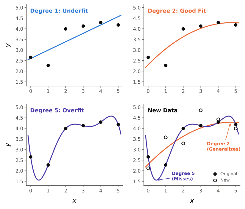
Figure: Three polynomials fit to the same six data points. The degree-1 line underfits (misses the curvature); the degree-2 quadratic captures the underlying trend; the degree-5 polynomial passes through every point exactly but oscillates wildly between them, having fit the noise rather than the signal. The fourth panel plots six new observations from the same process (open circles) where we find the overfit degree-5 misses them badly, while the simpler degree-2 quadratic still generalizes well. Passing through every training point is not the same as capturing the underlying relationship between variables.

Overfitting occurs when the model captures noise rather than signal. It shows up as a large gap between how well the model describes the data it was fit to (training error) and how well it predicts new data (test error). Adding parameters always improves training error but does not always improve (and often worsens) test error. This is especially important in behavior science, where datasets are often small (5-7 delay values in a discounting task, 5-10 prices in a demand assessment), so complex models with many free parameters can easily overfit. A high-degree polynomial fit to a handful of indifference points may explain 100% of the variance yet predict an absurd value (negative dollars, or more than the undiscounted reward) at an untested delay, whereas Mazur's hyperbolic (1 parameter), despite imperfect fit, predicts sensibly because its functional form encodes the known structure of discounting.

Parsimony (Occam's Razor)

Parsimony is the principle that, all else being equal, the simplest adequate model is preferred. This is sometimes called Occam's Razor and can be stated simply as, "Do not multiply entities beyond necessity". In modeling terms, do not add parameters beyond what the data justify.

Occam's Razor raises two questions: how do you quantify "simple", and how do you quantify "adequate"? The tools in this chapter answer them operationally. AIC and BIC formalize parsimony by imposing a penalty for each additional parameter. Cross-validation operationalizes adequacy by measuring predictive accuracy on held-out data. The bias-variance tradeoff explains why parsimony works. Every unnecessary parameter is an opportunity for the model to fit noise rather than signal.

Residuals and Residual Analysis

A residual is the difference between an observed value and the value predicted by a model:

$e_i = y_i - \hat{y}_i$

where $y_i$ is the observed value for data point $i$ and $\hat{y}_i$ is the model's prediction.

Residuals are the foundation of model evaluation. A good model produces residuals that are:

• Small in magnitude (the model's predictions are close to the data).
• Random in pattern (no systematic trends remain in what the model fails to capture).
• Homoscedastic (roughly equal in spread across the range of predicted values).

When residuals show systematic patterns (e.g., consistent overprediction at low values and underprediction at high values, a U-shaped pattern), this signals model misspecification. That is, the model is missing a feature a better model would capture. Residual analysis is therefore a diagnostic step before asking which model is "best".

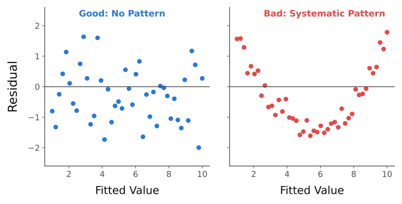
Figure: Residual analysis. Good residuals (left) scatter randomly around zero with no trend, indicating the model has captured the systematic structure of the data. Bad residuals (right) show a systematic pattern (here a U-shape) signaling model misspecification (i.e., there is some feature the model failed to capture). Overall error can look acceptable even when the residual pattern reveals the wrong functional form.

A simple diagnostic is the residual plot which is a scatterplot of residuals ($e_i$, y-axis) against predicted values ($\hat{y}_i$) or against values the independent variable took. Random scatter of residuals about zero indicates a well-specified model. Curvature, fanning, or other systematic deviations gotm random scatter indicates a problem. For example, an exponential fit to hyperbolic data overpredicts at short and long delays and underpredicts at intermediate delays, a red flag even when $r^2$ looks reasonable. The residual plot reveals that the functional form is wrong, not just imprecise.

Types of residual patterns and what they mean:

• Random scatter around zero: model well-specified; remaining error is noise.
• Curved pattern (U- or inverted-U-shaped): a missing nonlinear feature; consider a model with curvature.
• Fan-shaped (spread grows with predicted value): non-constant residual variance (heteroscedasticity); consider transforming the data or weighted regression.
• Trend (residuals rise or fall systematically): a missing linear component or misestimated slope.

Residual analysis should always come before any kind of numerical model comparison. There is no point computing AIC for a model whose residual plot reveals it is misspecified.

Variance Accounted For ($r^2$)

The coefficient of determination, $r^2$, quantifies the proportion of variance in the observed data that the model explains:

$r^2 = 1 - \frac{SS_{res}}{SS_{tot}}$

where:

• $SS_{res} = \sum_{i=1}^{N}(y_i - \hat{y}_i)^2$ is the residual sum of squares (variance left unexplained by the model).
• $SS_{tot} = \sum_{i=1}^{N}(y_i - \bar{y})^2$ is the total sum of squares (total variance in the data around its mean).

An $r^2$ of 0.90 means the model accounts for 90% of the variance; the remaining 10% could be measurement error, individual variability, or features the model does not capture.

$r^2$ is intuitive and widely used, but it has two critical limitations for model comparison. First, $r^2$ can never decrease when you add parameters. Adding a parameter gives the optimizer one more degree of freedom; at worst it sets the new parameter to a value with no effect (recovering the simpler model), so $SS_{res}$ cannot increase and $r^2$ cannot decrease. Second, $r^2$ has known inaccuracies with nonlinear models. Many phenomena in science are nonlinear in their input or output (more on this later).

Some researchers will also use an adjusted $r^2$, which imposes a penalty for additional parameters:

$r^2_{adj} = 1 - \frac{SS_{res} / (N - K)}{SS_{tot} / (N - 1)}$

where $N$ is the number of data points and $K$ is the number of estimated parameters. Adjusted $r^2$ can decrease when a new parameter does not improve fit enough to justify the added complexity, making it a better (though still imperfect) tool for model comparison.

As rough benchmarks, well-controlled laboratory data typically expect $r^2 > 0.85$, while applied settings (which have much less control) $r^2 > 0.60$ to $0.65$ is likely decent. These are guidelines, though, not critical cutoffs. The point is that obtaining an $r^2$ of 0.70 for a noisy clinical environment might be a greater achievement than 0.95 for a controlled pigeon experiment.

Loss Metrics

Beyond $r^2$, several loss metrics quantify how far a model's predictions are from the observed data. Each has its strengths and is appropriate in different contexts.

Mean Absolute Error (MAE): $MAE = \frac{1}{N} \sum_{i=1}^{N} |y_i - \hat{y}_i|$

MAE is the average absolute deviation between predicted and observed values. Its primary advantage is interpretability because it is expressed in the original units of the dependent variable. If you model indifference points in dollars, an MAE of $2.50 means predictions are off by $2.50 on average. MAE treats all errors equally regardless of sign or magnitude.

Mean Squared Error (MSE): $MSE = \frac{1}{N} \sum_{i=1}^{N} (y_i - \hat{y}_i)^2$

MSE squares each error before averaging. This makes causes large errors to be penalized disproportionately (e.g., being off by 10 on one point contributes 100 to the sum, while being off by 5 on two points contributes only 50). MSE is appropriate when large errors are especially undesirable, but its units are the square of the original units (e.g., dollars squared), making direct interpretation less intuitive.

Root Mean Squared Error (RMSE): $RMSE = \sqrt{MSE} = \sqrt{\frac{1}{N} \sum_{i=1}^{N} (y_i - \hat{y}_i)^2}$

RMSE takes the square root of MSE, returning to the original units while still penalizing large errors more heavily than MAE. It combines MSE's penalty structure with MAE's interpretability.

Comparing MAE and RMSE can itself be useful. When the two are close, errors are relatively uniform in size. When RMSE is much larger than MAE, a few points have disproportionately large errors, suggesting the model struggles with specific regions of the data.

An important limitation is that none of these loss metrics penalize complexity. A model with more parameters will often have equal or lower MAE, MSE, and RMSE on the data it was fit to. Like $r^2$, these loss metrics are necessary, but insufficient, for a complete model comparison. They measure how well the model fits, not whether the fit is achieved efficiently.

Akaike Information Criterion (AIC)

The Akaike Information Criterion addresses the limitations of raw fit metrics by explicitly penalizing model complexity:

$AIC = 2K - 2\ln(L)$

where:

• $K$ is the number of estimated parameters in the model.
• $L$ is the maximum likelihood of the data given the model (the probability of observing the data if the model, with its best-fitting parameters, were true).
• $\ln(L)$ is the natural logarithm of the likelihood.

Lower AIC is better. The term $-2\ln(L)$ measures lack of fit (smaller likelihood = worse fit = larger value). The term $2K$ is the complexity penalty. Each additional parameter adds 2 to the AIC regardless of how much it improves the likelihood, so a parameter is "worth" adding only if it improves the log-likelihood by more than 1 unit. AIC's information-theoretic foundation is that it estimates (up to a constant) the expected Kullback-Leibler divergence between the model and the true data-generating process (i.e., the information lost when the model approximates reality). The model with the lowest AIC loses the least information.

AIC differences ($\Delta$AIC) are often more informative than raw AIC values, which depend on sample size and data scale and are not interpretable in isolation. If Model A has AIC = 42 and Model B has AIC = 48, the difference is 6 units in favor of Model A. For context, here are some guidelines from Burnham and Anderson (2002):

• $\Delta$AIC $< 2$: Models are essentially equivalent; the data do not strongly distinguish them.
• $\Delta$AIC between 4 and 7: Some evidence favoring the model with lower AIC.
• $\Delta$AIC $> 10$: Significant evidence favoring the model with lower AIC.

For small samples (when $N/K < 40$, which is almost always true in behavioral research), a corrected version, AICc, is recommended:

$AICc = AIC + \frac{2K(K+1)}{N - K - 1}$

The extra penalty is negligible as $N$ grows but substantial when data are sparse: with $N = 6$ and $K = 2$ the correction term is $\frac{2 \cdot 2 \cdot 3}{6 - 2 - 1} = 4$, doubling the base complexity penalty. In behavioral research, where sample sizes are routinely single digits, AICc should generally be used instead of AIC.

Bayesian Information Criterion (BIC)

The Bayesian Information Criterion is similar to AIC but imposes a stronger penalty for complexity:

$BIC = K \cdot \ln(N) - 2\ln(L)$

where:

• $K$ is the number of estimated parameters.
• $N$ is the number of data points.
• $L$ is the maximum likelihood.

The key difference from AIC is the complexity penalty: $K \cdot \ln(N)$ instead of $2K$. Since $\ln(N) > 2$ whenever $N > 7$, BIC penalizes extra parameters more heavily than AIC for any reasonably sized dataset. And, because $\ln(N)$ grows with $N$ while $2K$ stays fixed, the two criteria can produce different rankings, especially with larger datasets.

Lower BIC is better, just as with AIC.

BIC has a Bayesian foundation as it approximates the log marginal likelihood (or "evidence"), which integrates over all parameter values weighted by their prior rather than evaluating only at the best-fitting values. This integration penalizes complex models more heavily, because their larger parameter spaces are mostly wasted on poor-fitting combinations. BIC therefore tends to favor simpler models than AIC, especially with large samples.

As a general rule of thumb, it can be useful to use AIC (or AICc) when your goal is predictive accuracy among models that are all approximations (the common situation in behavior science). And, to use BIC when you are trying to identify the "true" model and want a stronger guard against overfitting. Neither tells you the probability that a model is correct, and both rankings are relative to the candidate set. For example, if all candidates are poor, the "winner" is still poor. Always combine information criteria with residual analysis and substantive judgment.

Cross-Validation

Cross-validation takes a different approach. Instead of penalizing complexity mathematically, it measures predictive accuracy directly by evaluating the model on data it has never seen.

The basic idea is to create a hold out data set (the test set), fit the model to the rest (the training set), and evaluate predictions on the held-out data. A model that predicts the test set well generalizes. One that performs much worse on the test set than the training set is overfitting.

$k$-fold cross-validation systematizes this. To do $k$-fold cross-validation, divide the data into $k$ roughly equal folds, fit to the other $k-1$ folds and evaluate on each held-out fold. Repeate the process for every $k$ fold held out in turn. Then, average the prediction error across folds. Common choices are $k = 5$ or $k = 10$. Leave-one-out cross-validation (LOOCV) sets $k = N$, holding out one point at a time, which uses the maximum training data at each step.

Cross-validation penalizes complexity without an explicit penalty term. An overfit model has learned idiosyncratic features of the training points that are absent in held-out data, so its predictions suffer, while a simpler model that captured only the general trend generalizes better.

Cross-validation makes no assumptions about the form of the likelihood or penalty structure. Its limitation is that it requires enough data to split into meaningful training and test sets. With only 5 or 6 data points (common in discounting or demand tasks), each fold is tiny and a single held-out outlier can dominate the error estimate. For this reason, AIC and BIC are often preferred over cross-validation in behavior science, where sample sizes per individual are small. Cross-validation becomes more practical with group-level data or many conditions per participant.

Choosing Among Comparison Methods

Some practical guidelines:

• Standard comparison (2-4 candidate models, $N < 20$ per individual): use AICc as the primary criterion, report $r^2$ for descriptive context, and examine residual plots for every model.
• When AIC and BIC disagree: report both. Lean toward AIC if you need the most accurate predictions (e.g., a clinical application), toward BIC's more conservative selection if you want to claim something about the underlying process.
• When you have enough data: add cross-validation as a direct check on the AIC/BIC rankings.
• Always, regardless of sample size: generate and inspect residual plots. A model with the best AIC but systematic residuals is still misspecified.

The Bias-Variance Tradeoff

The bias-variance tradeoff is the conceptual framework that unifies all of the preceding tools. It explains why model comparison is necessary and why the best-fitting model is not always the best model.

Every model's prediction error can be decomposed into three components:

$\text{Total Error} = \text{Bias}^2 + \text{Variance} + \text{Irreducible Noise}$

• Bias is the systematic error from simplifying assumptions. A model that is too simple (e.g., a line fit to curved data) has high bias because its functional form cannot capture the true relationship, no matter how much data you collect. This is underfitting.
• Variance is the error from sensitivity to the particular dataset. A model that is too complex (e.g., a high-degree polynomial) fits very differently depending on which points happen to be in the sample, so its parameter estimates change dramatically across samples. This is overfitting.
• Irreducible noise is random variability no model can capture (measurement error, moment-to-moment fluctuations, and other out-of-scope sources).

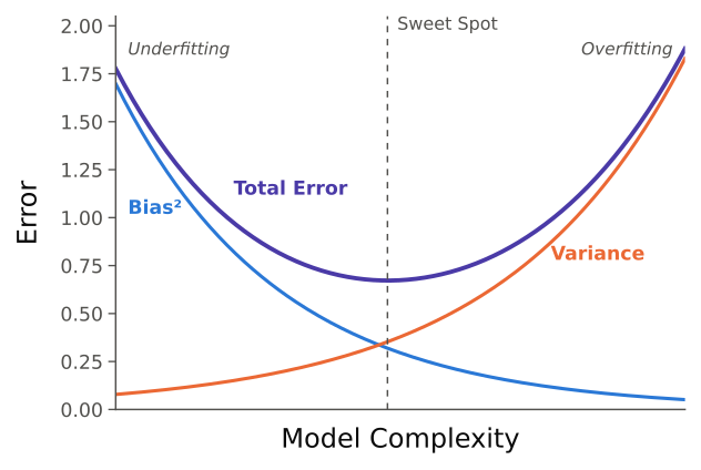
Figure: The bias-variance tradeoff. As model complexity increases, bias$^2$ falls (the model can capture more structure) while variance rises (the model chases sample-specific noise). Total error is their sum and is minimized at an intermediate complexity, the "sweet spot." Too simple underfits (high bias); too complex overfits (high variance). This is why the best-fitting model is not always the best model.

Bias and variance typically move in opposite directions as complexity changes. Simple models (few parameters) have high bias but low variance (i.e., they may miss real patterns but give stable estimates across samples). Complex models (many parameters) have low bias but high variance (i.e., they capture intricate patterns but fit noise, so estimates change across samples).

The optimal model minimizes total error by finding the sweet spot where the combined effect of bias and variance is smallest. This is precisely what AIC, BIC, and cross-validation attempt to identify, each from a different theoretical perspective. With the small sample sizes typical of single-subject research, variance is a particularly serious concern. A model with one too many free parameters can produce wildly different parameter estimates across conditions, undermining the generality of conclusions. Here, parsimony is a statistical necessity.

Each comparison tool maps onto the tradeoff differently: $r^2$ and loss metrics measure only fit (inversely related to bias) and ignore variance, which is why they always favor complexity. AIC's $2K$ penalty is a rough estimate of the variance contribution from $K$ parameters. BIC's stronger penalty guards more aggressively against variance at the cost of allowing more bias. And, cross-validation estimates total error directly, with both bias and variance driving poor performance on unseen data. This is why the tools sometimes disagree. Each makes different implicit tradeoffs between the cost of bias and the cost of variance.

---

Applying the 8-Step Framework

This week is a bit different since we're not really looking at deriving or using a model to describe or predict the relation between environmental variables and behavior. As such, we'll use the example below to show how we can use these model comparison techniques for various discounting models.

Let's say we have three candidate discounting models we want to compare.

Exponential discounting:

$V = A \cdot e^{-kD}$

This model has 1 free parameter ($k$), with $A$ known. It predicts a constant proportional decrease in value per unit delay, the same fraction of value lost per day whether the delay is 1 day or 100. It is the normative model from economics, following from a constant discount rate.

Mazur's hyperbolic discounting:

$V = \frac{A}{1 + kD}$

This model also has 1 free parameter ($k$). It produces the characteristic "hyperbolic" curve: steeper discounting at short delays, shallower at long delays. Unlike the exponential, it implies a decreasing discount rate (proportionally more value lost per unit time at short delays), which leads to the empirically documented preference reversals. It is the dominant descriptive model in behavior science (Mazur, 1987).

Myerson and Green's hyperboloid discounting:

$V = \frac{A}{(1 + kD)^s}$

This model has 2 free parameters ($k$ and $s$). When $s = 1$ it reduces to Mazur's hyperbolic; $s < 1$ makes the curve less bowed, $s > 1$ more bowed. The parameter $s$ controls curvature, accommodating individual differences in the shape of discounting. Because it nests the hyperbolic as a special case, the comparison is clean: is the extra parameter $s$ justified?

---

Worked Example

The Data

A participant completes a delay discounting task with a larger-later amount of A = \100$ at six delays. The indifference points are:

Delay (days)	Indifference Point ($)
1	95.0
7	82.0
30	55.0
90	30.0
180	18.0
365	10.0

These data show a clear pattern of declining subjective value with increasing delay, with the decline being steeper at shorter delays and shallower at longer delays, a pattern suggestive of hyperbolic rather than exponential discounting.

Fitting the Three Models

We use nonlinear least-squares regression to fit each model, minimizing $SS_{res} = \sum (y_i - \hat{y}_i)^2$.

Exponential model: $V = 100 \cdot e^{-0.0065 \cdot D}$, with $K = 1$

Delay	Observed	Predicted	Residual
1	95.0	99.35	-4.35
7	82.0	95.55	-13.55
30	55.0	82.27	-27.27
90	30.0	55.72	-25.72
180	18.0	31.04	-13.04
365	10.0	9.44	0.56

$SS_{res} = 4.35^2 + 13.55^2 + 27.27^2 + 25.72^2 + 13.04^2 + 0.56^2$ $SS_{res} = 18.92 + 183.60 + 743.65 + 661.52 + 170.04 + 0.31 = 1778.04$

The residuals are large and negative at intermediate delays, a systematic pattern showing the exponential decays too slowly at short delays and too quickly at intermediate ones, a clear sign of misspecification.

Hyperbolic model (Mazur): $V = \frac{100}{1 + 0.025 \cdot D}$, with $K = 1$

Delay	Observed	Predicted	Residual
1	95.0	97.56	-2.56
7	82.0	85.11	-3.11
30	55.0	57.14	-2.14
90	30.0	30.77	-0.77
180	18.0	18.18	-0.18
365	10.0	9.88	0.12

$SS_{res} = 6.55 + 9.67 + 4.58 + 0.59 + 0.03 + 0.01 = 21.44$

The residuals are dramatically smaller and show no systematic pattern. The largest residual is about 3 dollars, compared to 27 dollars for the exponential. The hyperbolic captures the shape of the data far better.

Hyperboloid model (Myerson & Green): $V = \frac{100}{(1 + 0.022 \cdot D)^{1.05}}$, with $K = 2$

Delay	Observed	Predicted	Residual
1	95.0	97.72	-2.72
7	82.0	85.84	-3.84
30	55.0	57.91	-2.91
90	30.0	30.47	-0.47
180	18.0	17.49	0.51
365	10.0	9.27	0.73

$SS_{res} = 7.40 + 14.75 + 8.47 + 0.22 + 0.26 + 0.53 = 31.63$

The hyperboloid with $s = 1.05$ fits slightly worse than the hyperbolic here: with $s$ so close to 1.0, it is essentially the hyperbolic with a slightly different $k$, and the extra parameter buys no meaningful improvement; the data do not require the added flexibility.

Computing $r^2$

First, compute $SS_{tot}$:

$\bar{y} = (95 + 82 + 55 + 30 + 18 + 10) / 6 = 290 / 6 = 48.33$

$SS_{tot} = (95 - 48.33)^2 + (82 - 48.33)^2 + (55 - 48.33)^2 + (30 - 48.33)^2 + (18 - 48.33)^2 + (10 - 48.33)^2$

$SS_{tot} = 2177.51 + 1132.45 + 44.49 + 336.09 + 919.71 + 1469.35 = 6079.60$

Now:

Model	$SS_{res}$	$R^2$
Exponential	1778.04	$1 - 1778.04/6079.60 = 0.708$
Hyperbolic	21.44	$1 - 21.44/6079.60 = 0.996$
Hyperboloid	31.63	$1 - 31.63/6079.60 = 0.995$

By $r^2$ alone, the hyperbolic and hyperboloid are nearly identical ($r^2 = 0.996$ vs. $0.995$), and both vastly outperform the exponential ($r^2 = 0.708$). But remember: $r^2$ does not account for the hyperboloid's extra parameter. We need AIC and BIC for a fair comparison.

Computing AIC and BIC

Under the assumption of normally distributed residuals, the log-likelihood for a model with $N$ observations and residual sum of squares $SS_{res}$ is:

$\ln(L) = -\frac{N}{2}\ln(2\pi) - \frac{N}{2}\ln\left(\frac{SS_{res}}{N}\right) - \frac{N}{2}$

We compute the full AIC and BIC using $N = 6$:

Exponential ($K = 1$):

• $\ln(SS_{res}/N) = \ln(1778.04/6) = \ln(296.34) = 5.691$
• $\ln(L) = -3\ln(2\pi) - 3(5.691) - 3 = -5.502 - 17.073 - 3 = -25.575$
• $AIC = 2(1) - 2(-25.575) = 2 + 51.15 = 53.15$
• $BIC = 1 \cdot \ln(6) - 2(-25.575) = 1.792 + 51.15 = 52.94$

Hyperbolic ($K = 1$):

• $\ln(SS_{res}/N) = \ln(21.44/6) = \ln(3.573) = 1.274$
• $\ln(L) = -3\ln(2\pi) - 3(1.274) - 3 = -5.502 - 3.822 - 3 = -12.324$
• $AIC = 2(1) - 2(-12.324) = 2 + 24.648 = 26.65$
• $BIC = 1 \cdot \ln(6) - 2(-12.324) = 1.792 + 24.648 = 26.44$

Hyperboloid ($K = 2$):

• $\ln(SS_{res}/N) = \ln(31.63/6) = \ln(5.272) = 1.663$
• $\ln(L) = -3\ln(2\pi) - 3(1.663) - 3 = -5.502 - 4.989 - 3 = -13.491$
• $AIC = 2(2) - 2(-13.491) = 4 + 26.982 = 30.98$
• $BIC = 2 \cdot \ln(6) - 2(-13.491) = 3.584 + 26.982 = 30.57$

Computing AICc

Given the small sample size ($N = 6$), we should also compute AICc:

Exponential ($K = 1$): $AICc = 53.15 + \frac{2(1)(2)}{6 - 1 - 1} = 53.15 + 1.0 = 54.15$

Hyperbolic ($K = 1$): $AICc = 26.65 + \frac{2(1)(2)}{6 - 1 - 1} = 26.65 + 1.0 = 27.65$

Hyperboloid ($K = 2$): $AICc = 30.98 + \frac{2(2)(3)}{6 - 2 - 1} = 30.98 + 4.0 = 34.98$

Notice that AICc increases the hyperboloid's penalty substantially (from 30.98 to 34.98), widening the gap between the hyperbolic and hyperboloid. With small $N$, the cost of extra parameters is higher.

Summary Table

Model	$K$	$R^2$	$SS_{res}$	AIC	AICc	BIC
Exponential	1	0.708	1778.04	53.15	54.15	52.94
Hyperbolic	1	0.996	21.44	26.65	27.65	26.44
Hyperboloid	2	0.995	31.63	30.98	34.98	30.57

Interpretation

The hyperbolic wins decisively on every metric. Against the exponential it has $\Delta$AIC = 26.5 and $\Delta$BIC = 26.5, overwhelming evidence; the exponential cannot capture the shape of these data ($R^2 = 0.708$, systematic residuals). The more interesting comparison is hyperbolic vs. hyperboloid: the hyperbolic has lower AIC by 4.33 units and lower BIC by 4.13, and under AICc (more appropriate for $N = 6$) the gap widens to 7.33. All criteria favor the simpler model, because the hyperboloid's extra parameter ($s = 1.05 \approx 1$, the hyperbolic special case) buys virtually no improvement.

The key principle: the hyperboloid is not a "worse" model in general; it is simply unnecessary for this dataset. For a participant whose function deviates more from the standard hyperbolic shape ($s$ far from 1), it might win. Model comparison is always relative to the data at hand.

Computing Loss Metrics

For completeness, we compute MAE and RMSE for each model:

Model	MAE	RMSE
Exponential	$(4.35 + 13.55 + 27.27 + 25.72 + 13.04 + 0.56)/6 = 14.08$	$\sqrt{1778.04/6} = 17.22$
Hyperbolic	$(2.56 + 3.11 + 2.14 + 0.77 + 0.18 + 0.12)/6 = 1.48$	$\sqrt{21.44/6} = 1.89$
Hyperboloid	$(2.72 + 3.84 + 2.91 + 0.47 + 0.51 + 0.73)/6 = 1.86$	$\sqrt{31.63/6} = 2.30$

The hyperbolic's MAE of $1.48 means predictions are off by less than $1.50 on average, with RMSE ($1.89) close to MAE, indicating uniform error. The exponential's MAE of $14.08 (off by more than $14 on average) is clearly inadequate.

The RMSE-to-MAE ratios are all near 1.2--1.3 (exponential $17.22/14.08 = 1.22$, hyperbolic $1.89/1.48 = 1.28$, hyperboloid $2.30/1.86 = 1.24$), indicating relatively uniform residual sizes in each model rather than one point dominating.

What Would Make the Hyperboloid Win?

The hyperboloid would be preferred for a participant whose discounting function is noticeably more bowed than the standard hyperbolic, indifference points that drop very steeply at short delays and then flatten more than the hyperbolic predicts. For such data $s$ would land well away from 1.0 (say, $s = 0.6$ or $s = 1.5$), and the improved fit would overcome the AIC/BIC penalty. The "right" model depends on the individual's data. For example, across 50 participants the hyperbolic might describe data best for most but the hyperboloid or exponential for some, so reporting model comparison at the individual level (not just group level) avoids masking real individual differences.

Making a Prediction

The payoff of model selection is reliable prediction. Having selected the hyperbolic model with $k = 0.025$, we can predict indifference points at untested delays:

• At $D = 14$ days: V = 100 / (1 + 0.025 \times 14) = 100 / 1.35 = \74.07$
• At $D = 500$ days: V = 100 / (1 + 0.025 \times 500) = 100 / 13.5 = \7.41$
• At $D = 730$ days (2 years): V = 100 / (1 + 0.025 \times 730) = 100 / 19.25 = \5.19$

These predictions are only as good as the model choice: the exponential (with $r^2 = 0.708$ and systematic residuals) would give unreliable ones. Model comparison is what makes these predictions trustworthy.

---

Exercises for Reflection

1. A colleague fits a 4-parameter model to a dataset with 6 data points and reports $r^2 = 0.99$. They claim the model provides an excellent account of the data. What concerns would you raise, and what additional analyses would you recommend? How would you explain the problem to someone who is not familiar with overfitting?

2. You are comparing two models of demand: the exponential model (2 parameters: $Q_0$ and $\alpha$) and a modified model with an additional shape parameter (3 parameters). AIC favors the 3-parameter model, but BIC favors the 2-parameter model. How would you interpret this disagreement, and what would you recommend? Under what circumstances might you side with AIC, and under what circumstances with BIC?

3. Consider the bias-variance tradeoff in the context of single-subject research. With data from a single participant across 5 conditions, how does the small sample size affect the tradeoff? Would you generally lean toward simpler or more complex models in this context, and why? How might your answer change if you had data from 50 conditions?

4. A research team uses cross-validation to compare models and finds that the hyperbolic discounting model has lower cross-validated RMSE than the exponential model, but higher cross-validated RMSE than the hyperboloid model. However, AIC and BIC both favor the hyperbolic. How would you reconcile these findings? What might explain the discrepancy between cross-validation and information criteria in this case?

---

Key Readings

Required:

Chapter 6 from Cox and Vladescu (2023) provided a practical primer on interpreting the output of fitted models, covering residual analysis, variance accounted for ($r^2$), mean absolute error, mean squared error, root mean squared error, AIC, and BIC. They explained when each metric is appropriate---$r^2$ for linear models, information criteria when comparing models of different complexity---and emphasized the distinction between a model that fits the training data well and a model that will generalize to new data. This chapter is the methodological foundation for the week: it gives students the concrete tools they need to evaluate and compare every model encountered in the course, and it makes the abstract principle of parsimony operational through specific fit metrics.

Mazur (2001) compared three quantitative models of animal choice---the hyperbolic value addition model, the contextual choice model, and the incentive theory model---across concurrent-chain and variable-delay procedures. He evaluated each model not just on overall fit but on its ability to handle specific empirical patterns that competing models could not accommodate. The paper exemplifies the model-comparison process that is this week's central topic: rather than asking which model fits best on a single dataset, Mazur asked which model provides the most consistent account across diverse experimental conditions, demonstrating that model comparison is about generality, not just goodness of fit.

Supplemental:

Mazur (2006) offered a broader reflection on the role of mathematical models in the experimental analysis of behavior, discussing what makes a model useful, how models relate to theories, and what standards should govern model evaluation. He argued that models should be judged not only by their quantitative fit but by their ability to organize existing findings and generate novel predictions. This paper provides philosophical context for the week's technical material, grounding the fit metrics and comparison tools in a larger vision of what the modeling enterprise is trying to accomplish.

McDowell (2005) contrasted the classic matching theory (Herrnstein's original formulation) with modern matching theory (the generalized matching equation and its computational extensions), evaluating their relative strengths and weaknesses as accounts of concurrent-schedule performance. He used this comparison to illustrate broader principles of model evaluation, including the importance of parameter interpretability, the danger of post hoc modifications, and the value of deriving predictions from first principles rather than fitting flexible functions to data. This paper provides a concrete case study in model comparison using the matching law---a model students have already studied---making the week's abstract tools tangible.

---

Reading Guide

Chapter 6 from Cox & Vladescu (2023)

• What are the two phases involved in interpreting the output of a statistical model?
• What does a "loss metric" represent in the context of model evaluation? Why is it needed?
• Why is the raw data considered the most accurate description of observed behavior? What is the tradeoff in using a model instead?
• What are residuals, and how are they calculated from observed and predicted values? What does a residual plot display, and what should it ideally look like for a good model fit?
• What might it indicate if residuals show a systematic trend as the IV increases?
• What is variance accounted for ($r^2$ or VAC), and how is it calculated from residuals?
• When is $r^2$ an appropriate fit metric, and why is it not suitable for nonlinear models?
• As a rule of thumb, what value of $r^2$ would be considered acceptable in (a) experimental lab settings, and (b) complex applied settings?
• What is mean absolute error (MAE), and why might it be preferred for nonlinear models?
• How is mean squared error (MSE) different from MAE, and what tradeoffs does it involve?
• What is root mean squared error (RMSE), and how does it combine benefits of both MSE and MAE?
• What limitation do MAE, MSE, and RMSE share when comparing model complexity?
• What are AIC and BIC, and what do they add to our understanding of model performance beyond loss?
• How does AIC penalize model complexity, and how is this different from BIC?
• When would you choose BIC over AIC in a model comparison?
• Why is it important to balance model fit with parsimony (Occam's Razor) in behavior analysis?
• What is accuracy in classification models, and when is it appropriate as a fit metric?
• What alternative metrics might be better than accuracy when dealing with imbalanced classes or asymmetric errors?

Mazur (2001)

• What are the two major goals of a general model of animal choice, according to Mazur?
• What are the "three main procedures used to study animal choice" described by the author? What are your reactions to these three preparations being the dominant methods to study "animal choice"?
• What are the three quantitative models compared in this article? Be able to state their name, provide the equation, and identify what each parameter represents.
• What data were used to compare the three models for concurrent-chain performance? What fit metric was used? What were the results?
• What data were used to compare the models for choice between fixed and variable terminal links? What fit metric was used? What were the results?

---

References

Burnham, K. P., & Anderson, D. R. (2002). Model selection and multimodel inference: A practical information-theoretic approach (2nd ed.). Springer.

Cox, D. J., & Vladescu, J. C. (2023). Statistics for applied behavior analysis practitioners and researchers. Academic Press.

Hursh, S. R., & Silberberg, A. (2008). Economic demand and essential value. Psychological Review, 115(1), 186--198. https://doi.org/10.1037/0033-295X.115.1.186

Mazur, J. E. (1987). An adjusting procedure for studying delayed reinforcement. In M. L. Commons, J. E. Mazur, J. A. Nevin, & H. Rachlin (Eds.), Quantitative analyses of behavior: Vol. 5. The effect of delay and of intervening events on reinforcement value (pp. 55--73). Erlbaum.

Mazur, J. E. (2001). Hyperbolic value addition and general models of animal choice. Psychological Review, 108(1), 96--112. https://doi.org/10.1037/0033-295X.108.1.96

Mazur, J. E. (2006). Mathematical models and the experimental analysis of behavior. Journal of the Experimental Analysis of Behavior, 85(2), 275--291. https://doi.org/10.1901/jeab.2006.65-05

McDowell, J. J. (2005). On the classic and modern theories of matching. Journal of the Experimental Analysis of Behavior, 84(1), 111--127. https://doi.org/10.1901/jeab.2005.59-04

Myerson, J., & Green, L. (1995). Discounting of delayed rewards: Models of individual choice. Journal of the Experimental Analysis of Behavior, 64(3), 263--276. https://doi.org/10.1901/jeab.1995.64-263

---

Key Takeaways

• Overfitting occurs when a model captures noise rather than signal. Adding parameters always improves fit to the training data but can worsen predictions for new data. With the small sample sizes common in behavior science, overfitting is a constant concern.
• Parsimony (Occam's Razor) favors the simplest model that adequately describes the data. AIC and BIC formalize this principle by imposing mathematical penalties for model complexity.
• Residual analysis is a diagnostic tool that should precede numerical model comparison: systematic patterns in residuals signal model misspecification, regardless of $R^2$ or other summary metrics.
• $R^2$ quantifies variance explained but always increases with more parameters, making it insufficient alone for model comparison. Use adjusted $R^2$ or information criteria instead.
• Loss metrics (MAE, MSE, RMSE) measure prediction error in interpretable units but do not penalize complexity. They are useful for communicating model accuracy but cannot distinguish between a good model and an overfitting model.
• AIC ($2K - 2\ln(L)$) balances fit against complexity with an information-theoretic foundation. Lower is better. Use AICc for small samples (which is almost always in behavior science).
• BIC ($K \cdot \ln(N) - 2\ln(L)$) imposes a stronger complexity penalty than AIC and is preferred when avoiding overfitting is the priority. Lower is better.
• Cross-validation directly measures predictive accuracy on unseen data without relying on mathematical penalties, but requires sufficient data to be reliable.
• The bias-variance tradeoff explains why model comparison is necessary: simple models are biased but stable; complex models are flexible but noisy. The best model minimizes total error by finding the sweet spot.
• Model comparison is always relative: it identifies the best model among those considered, not the "true" model. All candidates might be inadequate, and the comparison is only as good as the candidate set.
• In behavior science, model comparison is standard practice in discounting (Mazur, 2001, 2006), matching (McDowell, 2005), demand, and learning research. Reporting AIC/BIC alongside $R^2$ is increasingly expected in quantitative behavioral publications.