Week 5: Behavioral Momentum and Response Persistence

Why This Topic Matters

Learning a predictive relation is only part of the story; another is how persistently the resulting behavior holds up when conditions change. A pigeon does not stop pecking the moment the contingency changes, and a child's reinforced tantrums do not stop the moment a new intervention begins. The degree to which behavior persists is predictable, quantifiable, and governed by identifiable variables.

This is the domain of behavioral momentum theory (BMT). BMT draws an explicit analogy to Newtonian mechanics: behavior has a velocity (its rate of occurrence) and a mass (its resistance to change when a disruptor is applied). Just as a heavier object is harder to stop, behavior maintained in a richer reinforcement context is harder to disrupt. The key result is that rate and persistence are influenced by different variables. A behavior can occur at a low rate yet persist for long periods, while another can occur at a high rate yet collapse quickly under disruption. This distinction matters for any intervention: reducing a problem behavior, building durable replacement behaviors, or predicting relapse all require knowing both what maintains behavior and how resistant it will be to change.

Behavioral momentum extends the Week 4 logic to a different level of analysis. Where Rescorla-Wagner asks how an individual CS-US association forms, BMT asks how the overall Pavlovian relationship between a discriminative stimulus context and reinforcement determines the persistence of behavior in that context. The bridge between the two is the Pavlovian contingency: Week 4 formalized how it builds associative strength; this week we see how it builds behavioral persistence.

Core Concepts

Behavioral Momentum Theory

Behavioral momentum theory (BMT) provides a formal account of how resistant behavior is to disruption. The theory draws an explicit analogy to Newtonian mechanics: just as a moving object with greater mass is harder to stop, behavior maintained in a richer reinforcement context is harder to disrupt.

Response rate is controlled primarily by the response-reinforcer contingency (i.e., the operant relation). How often you press the lever per minute depends on the schedule of reinforcement for lever pressing. Resistance to change, by contrast, is controlled primarily by the stimulus-reinforcer contingency (i.e., the respondent relation between the discriminative stimulus and all reinforcement obtained in its presence, regardless of whether that reinforcement is contingent on the target response).

This distinction was originally demonstrated using multiple schedules. In a typical design, pigeons respond in two components of a multiple schedule. Both components have identical response-reinforcer contingencies (e.g., the same VI schedule), but one component includes additional response-independent (free) food deliveries. The free food does not increase response rate. But when disruption is introduced (e.g., pre-feeding, extinction), behavior in the component with additional food is more resistant to change. The free food added to the learned stimulus-reinforcer relation (more total food in the presence of that stimulus) without changing the response-reinforcer relation.

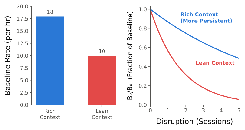
Rate and resistance are dissociable

Figure: A richer reinforcement context supports both more responding and greater persistence. The rich context maintains a higher baseline response rate (left), and its behavior is far more resistant to disruption (right): as a fraction of baseline, responding decays toward zero much more slowly. Resistance to change is governed by the total reinforcement obtained in the stimulus context (the Pavlovian relation), which is what makes the richer context harder to disrupt.

The basic quantitative expression for resistance to change is:

$\log \left( \frac{B_x}{B_o} \right) = -x \cdot \frac{c}{r}$

where:

$B_o$ is the baseline response rate before disruption
$B_x$ is the response rate during or after disruption
$x$ is the magnitude of the disruptor (e.g., duration of pre-feeding, number of extinction sessions)
$r$ is the rate of reinforcement in the component during baseline
$c$ is a scaling constant that captures the effectiveness of the disruptor

The ratio $B_x / B_o$ is the proportional change in behavior. Taking the logarithm means we are modeling proportional change on a log scale, which is standard practice when comparing across conditions with different baselines.

In plain language: the proportional change in behavior during disruption is a function of the ratio of disruption magnitude to reinforcement rate. Higher reinforcement rates produce less proportional change (i.e., greater momentum) because the behavior has more "mass".

The Pavlovian / Respondent Nature of Behavioral Momentum

A commonly misunderstood point is worth stating explicitly: resistance to change is fundamentally a respondent (Pavlovian) phenomenon, not an operant one. The intuition that "more-reinforced behavior is stronger and harder to reduce" conflates two things that reinforcement in the presence of a discriminative stimulus does at once: it maintains the operant response (the response-reinforcer contingency, which controls rate), and it establishes a Pavlovian association between the stimulus context and reinforcement (the stimulus-reinforcer contingency, which controls resistance to change). The free-reinforcer result dissociates them: adding response-independent food, which is not contingent on any response, increases resistance to change even though it does not raise rate. What we observe as the "persistence of operant behavior" is driven by the respondent association between the discriminative stimulus and reinforcement, regardless of that reinforcement's source.

The clinical implication follows directly. To make a replacement behavior more durable, reinforce it more often (to raise rate) and ensure its context is richly associated with reinforcement from all sources. To make a problem behavior less persistent, reducing the overall reinforcement in its context may be more effective than changing the operant contingency alone.

The Augmented Model of Behavioral Momentum

The basic momentum equation describes how behavior changes proportionally to the ratio of disruption to reinforcement rate. But subsequent research revealed that additional factors also matter. This work led to augmented models of behavioral momentum.

One important extension considers the role of the reinforcer-response contingency in modulating resistance to change. While the basic model treats all reinforcement in a context as equivalent (whether contingent on the target response or not), augmented models allow for the the source of reinforcement to matter.

The augmented model can be expressed as: $\log \left( \frac{B_x}{B_o} \right) = -x \cdot \frac{c}{r_c + a \cdot r_o}$ where:

$r_c$ is the rate of contingent reinforcement (reinforcers contacted by the target response)
$r_o$ is the rate of other (non-contingent) reinforcement in the context
$a$ is a parameter that weights the contribution of non-contingent reinforcement relative to contingent reinforcement
The remaining parameters are as in the basic model.

When $a = 1$ , all reinforcement contributes equally to behavioral mass, and the model reduces to the basic version. When $a < 1$ , contingent reinforcement contributes more to resistance to change than non-contingent reinforcement. This captures the empirical finding that while both sources of reinforcement contribute to momentum, contingent reinforcement may have a somewhat larger effect per unit.

Key Predictions of Behavioral Momentum Theory

The framework generates several important predictions:

Differential resistance to change: In a multiple schedule with rich and lean components, behavior in the rich component will be proportionally less disrupted by extinction, satiation, or other challenges. This has been confirmed repeatedly.
Independence of rate and resistance: Manipulations that change response rate (e.g., adding a response cost) do not necessarily change resistance to change. And manipulations that change resistance to change (e.g., adding free reinforcers) do not necessarily change response rate.
Clinical implications for problem behavior: If a problem behavior occurs in a context rich in reinforcement (e.g., a child's tantrums are reinforced by attention in a context that also includes many other reinforcers), that behavior will be resistant to treatment-induced disruption.
Relapse prediction: When treatment is itself disrupted (e.g., a caregiver stops implementing an intervention, or the individual moves to a new setting), the original problem behavior may resurge. Behavioral momentum theory, extended to a quantitative model of resurgence (Shahan & Craig, 2017), predicts the degree of relapse based on the reinforcement history of the problem behavior and the treatment context.

The physics metaphor is worth examining carefully. In Newtonian mechanics, momentum = mass $\times$ velocity, and force = mass $\times$ acceleration. A heavier object requires more force to change its velocity by a given amount. In behavioral momentum theory, "mass" corresponds to the strength of the stimulus-reinforcer relation (the respondent context), "velocity" corresponds to response rate, and "force" corresponds to the disruptor.

However, the metaphor has limits. In physics, momentum is a conserved quantity in closed systems. In behavior, there is no conservation law. Reinforcement can be added or removed without known compensating changes elsewhere. The metaphor guides thinking but should not be taken literally beyond its intended scope.

Applying the 8-Step Framework

This section walks through each step of the 8-step modeling framework using BMT applied to a clinical scenario: predicting resistance to change of problem behavior in rich versus lean reinforcement contexts during treatment.

Step 1: Identify All Environmental and Behavioral Components of the Phenomenon A child, Alex, engages in disruptive behavior (loud vocalizations and throwing materials) across two classroom settings. In Setting A (the general education classroom), Alex receives frequent adult attention contingent on disruption (teacher redirections, verbal reprimands) and non-contingent (frequent check-ins, proximity to the aide, group praise). The total rate of reinforcement (all attention combined) in Setting A is approximately 40 reinforcers per hour. In Setting B (the resource room), Alex works one-on-one with a paraprofessional who delivers attention primarily contingent on disruption (redirection after each episode) but provides little non-contingent attention. The total reinforcement rate in Setting B is approximately 10 reinforcers per hour.

Baseline data show that Alex's disruption rate is similar across both settings at approximately 8 episodes per hour in Setting A and 10 episodes per hour in Setting B. A new intervention is introduced simultaneously in both settings. These are planned ignoring of disruption (extinction) combined with differential reinforcement of alternative behavior (DRA).

The clinical team wants to predict: In which setting will the disruptive behavior be more resistant to the intervention? How much residual disruption should they expect after the first week of treatment in each setting?

Step 2: Define the Behavioral Principles, Processes, and Intended Scope of the Model We are modeling the resistance to change of disruptive behavior when an extinction-based intervention is introduced. The model's scope includes:

How the proportional change in disruption rates differs between the two settings as a function of their reinforcement histories.
How the magnitude of disruption relates to the reinforcement rate in each context.

We are explicitly NOT modeling:

The specific topography of disruptive behavior
The acquisition of the alternative (replacement) behavior
Moment-to-moment fluctuations in behavior within sessions
Motivating operations or setting events that may vary across days
The caregiver's fidelity to the intervention protocol
Long-term maintenance or generalization

Step 3: Write Down the Behavioral Principles, Known Quantitative Laws, and Functional Relationships The governing principle is that resistance to change is determined by the Pavlovian stimulus-reinforcer relationship in the discriminative stimulus context. That is, the total rate of reinforcement obtained in the presence of the setting cues, regardless of whether that reinforcement is contingent on the target response.

The quantitative law is the behavioral momentum equation: $\log \left( \frac{B_x}{B_o} \right) = -x \cdot \frac{c}{r}$

This states that the proportional decline in behavior (on a log scale) is a linear function of the disruption magnitude, scaled by the ratio of the disruptor's effectiveness to the reinforcement rate in the context.

Step 4: State All Simplifying Assumptions Explicitly

All reinforcement in a context contributes equally to behavioral mass (we use the basic model rather than the augmented model, so $a = 1$ ).
The reinforcement rate during baseline is a stable, representative estimate of the Pavlovian S-SR+ relationship.
The disruptor (extinction + DRA) operates uniformly across both settings with equal effectiveness.
The scaling constant $c$ is the same in both settings (the disruptor itself does not differ between contexts).
Baseline response rates are stable and representative.
The model applies to the proportional change in the target behavior only; it does not predict the absolute level of the replacement behavior.
No other major variables (illness, medication changes, schedule changes) influence behavior change during the treatment period.

Step 5: Write the Model Verbally, Then Express It Mathematically Verbally: When the extinction-based intervention is introduced, the challening behavior will decrease in both settings. However, the proportional decline will be greater in Setting B (lean context) than in Setting A (rich context), because Setting A has a greater Pavlovian association between the setting cues and reinforcement. The richer reinforcement history in Setting A gives the disruptive behavior more "mass" (i.e., more resistance to the intervention's disruptive force). After a given duration of treatment, disruption in Setting A will retain a larger proportion of its baseline level than disruption in Setting B.

Mathematically: $\log \left( \frac{B_x}{B_o} \right) = -x \cdot \frac{c}{r}$

where:

$B_o$ (Setting A) = 8 episodes/hr; $B_o$ (Setting B) = 10 episodes/hr
$r$ (Setting A) = 40 reinforcers/hr; $r$ (Setting B) = 10 reinforcers/hr
$x$ = number of treatment sessions (our unit of disruption magnitude)
$c$ = 8 (a scaling constant we estimate from prior clinical data or the literature, representing the effectiveness of the extinction + DRA combination per session)

Step 6: Verify Dimensional Consistency $B_x$ and $B_o$ are both in responses per hour, so their ratio is dimensionless, and the log of a dimensionless ratio is dimensionless. On the right side, $x$ is in sessions, $c$ is in reinforcers/hr per session (a rate constant), and $r$ is in reinforcers/hr. The ratio $c/r$ is therefore dimensionless per session, and $x \cdot c/r$ is dimensionless. Both sides are dimensionless. The equation is consistent.

Step 7: Specify Starting Values and Constraints

$B_o$ (Setting A) = 8 episodes/hr; $B_o$ (Setting B) = 10 episodes/hr
$r$ (Setting A) = 40; $r$ (Setting B) = 10
$c = 8$ (estimated; in practice, this would be fit to early treatment data)
$x \geq 0$ : disruption magnitude cannot be negative
$B_x / B_o$ is bounded between 0 and 1 (behavior cannot go below zero or exceed baseline during extinction)
The model applies from the onset of treatment ( $x = 0$ ) onward

Step 8: Check the Math, Test Against Data, and Derive Predictions Compute predictions for $x = 5$ treatment sessions: Setting A (rich context): $\log \left( \frac{B_x}{8} \right) = -5 \times \frac{8}{40} = -5 \times 0.2 = -1.0$ $\frac{B_x}{8} = 10^{-1.0} = 0.10$ $B_x = 0.80 \text{ episodes/hr}$

Disruption in Setting A drops from 8 to 0.8 episodes per hour (~10% of baseline). A substantial reduction, but not elimination.

Setting B (lean context): $\log \left( \frac{B_x}{10} \right) = -5 \times \frac{8}{10} = -5 \times 0.8 = -4.0$ $\frac{B_x}{10} = 10^{-4.0} = 0.0001$ $B_x = 0.001 \text{ episodes/hr}$

Disruption in Setting B leads to essentially elimination of responding (i.e., reduced to less than one-thousandth of its baseline level).

Comparison: After 5 sessions of the same intervention, Setting A retains 10% of baseline disruption while Setting B retains 0.01%. The four-fold difference in reinforcement rate produces a signifiant difference in persistence. This is the core prediction of behavioral momentum theory: the richer Pavlovian context in Setting A gives the disruptive behavior more mass, making it substantially harder to eliminate.

Boundary check: At $x = 0$ , both settings predict $B_x / B_o = 1$ (no change before treatment begins). As $x \to \infty$ , both predict $B_x \to 0$ (eventually behavior is eliminated). These are sensible.

Clinical implication: The treatment team should expect slower progress in Setting A and should prepare for the possibility that disruption will persist longer there. They might consider strategies to reduce the overall reinforcement density in Setting A (e.g., thinning non-contingent attention) to reduce the behavioral mass of the problem behavior before or during treatment.

Derive new predictions:

If the intervention is temporarily suspended (e.g., a substitute teacher does not implement the protocol), behavioral momentum theory predicts that disruption will recover more in Setting A than in Setting B, because the underlying Pavlovian association is greater.
If a new reinforcer is introduced in Setting B (e.g., access to a preferred activity), it will increase the overall S-SR+ relationship and increase the momentum of all behavior in that context including the target behavior.

Connection to Empirical Behavior Science

Nevin and colleagues (Nevin et al., 1983) established the foundational findings using multiple schedules with pigeons: behavior in the component with the higher reinforcement rate was more resistant to disruption by pre-feeding, extinction, or alternative reinforcement. These findings have replicated across species (pigeons, rats, humans), response types, and disruptors, and that generality is one of the theory's greatest strengths.

Clinically, the same framework predicts (a) treatment relapse and resurgence, where a problem behavior maintained in a rich context is more likely to re-emerge when treatment contingencies are disrupted; (b) an FCT paradox, where training a communication response in a richer context makes it more durable but also increases the momentum of any residual problem behavior in that context; and (c) context effects, where conducting treatment in a novel or leaner context, rather than where the problem behavior was historically reinforced, can reduce its momentum. In each case the practical lesson is the same: many intervention failures reflect an underappreciated Pavlovian context rather than an inadequate operant contingency.

Assumptions and Limitations

Behavioral momentum theory, like all models, rests on assumptions that constrain its applicability:

Log-linear relationship: The model assumes that the log-proportional change in behavior is a linear function of disruption magnitude. This is an approximation that holds well for moderate disruption but may break down at extremes (very small or very large disruptors).
Aggregate-level analysis: The model describes group-level or condition-level trends. It does not predict trial-by-trial or moment-to-moment fluctuations in behavior. Individual sessions may deviate substantially from the predicted trajectory.
Static reinforcement rate: The model uses a single reinforcement rate to characterize each context. In reality, reinforcement rates may fluctuate across sessions, and the effective reinforcement rate may change as the organism's behavior changes during disruption.
No conservation law: Unlike physical momentum, behavioral momentum is not known to be conserved. The metaphor is productive but not literal. Adding reinforcement to a context increases behavioral mass without requiring a corresponding decrease elsewhere.
Limited scope of the basic model: The basic equation does not account for the source of reinforcement (contingent vs. non-contingent), the type of reinforcer, or the organism's motivational state. The augmented model addresses some of these limitations but adds parameters.
Extinction is not a pure disruptor: Extinction changes the operant contingency (removing reinforcement for the target response), which means it is not purely an external "force" applied to behavior. This has been debated in the literature, and some researchers argue that extinction-induced disruption confounds operant and Pavlovian effects.
No representation of behavioral variability: The model predicts the central tendency of behavior under disruption but does not predict the increase in behavioral variability (extinction bursts, novel response forms) that typically accompanies disruption.

These limitations define where the model applies and where extensions are needed. The theory's strength lies in its ability to generate clear, testable, quantitative predictions about resistance to change (a single phenomenon) that is otherwise difficult to formalize.

Exercises for Reflection

A therapist is implementing functional communication training (FCT) for a client whose hand-biting is maintained by escape from demands. The FCT is conducted in two settings: a clinic room (lean context, few other reinforcers available) and the client's classroom (rich context, many other reinforcers available throughout the day). Using behavioral momentum theory, predict which setting will show (a) faster initial reduction of hand-biting, and (b) more durable maintenance of the communication response. Is there a tension between these two goals? Explain.
Behavioral momentum theory claims that resistance to change is determined by the stimulus-reinforcer (Pavlovian) relationship, not the response-reinforcer (operant) relationship. Design a thought experiment that would allow you to test this claim. Specify two conditions that have the same operant contingency but different Pavlovian associations, describe the disruption you would introduce, and state what the theory predicts about resistance to change in each condition. What would it mean for the theory if the two conditions showed equal resistance to change?
Consider the phenomenon of resurgence: a previously reinforced response re-emerges when alternative reinforcement is removed. Use the behavioral momentum framework to explain why resurgence occurs. Then consider: if you were designing an FCT intervention and wanted to minimize the risk of resurgence when treatment contingencies are eventually thinned, what would behavioral momentum theory recommend? Think about both the treatment phase (Phase 2) and the transition to maintenance (Phase 3).
The physics metaphor in behavioral momentum theory is powerful but imperfect. Identify two ways in which behavioral momentum differs from physical momentum. For each difference, explain whether it is a minor limitation (the metaphor is still useful) or a fundamental problem (the metaphor is misleading). How should we treat metaphors in formal modeling (e.g., as heuristics, as structural guides to theory construction, something else)?

Key Readings

Required: Nevin, Mandell, and Atak (1983) presented the foundational empirical and quantitative analysis of behavioral momentum, demonstrating that resistance to change is a function of the reinforcement context rather than the response-reinforcer contingency alone. Using multiple-schedule procedures with pigeons, they showed that behavior in components with higher reinforcement rates was more resistant to disruption by extinction and response-independent food, even when baseline response rates were similar or lower. The paper formalized the analogy to Newtonian momentum, with response rate as velocity and resistance to change as mass, and introduced the quantitative methods that became standard in the field (i.e., log-proportion change, lateral shift analysis).

Supplemental: Nevin (1998) connected behavioral momentum theory to choice, arguing that the persistence of behavior in a given context can be understood through the same Pavlovian stimulus-reinforcer relationships that govern preference in concurrent schedules. He showed that momentum and choice are not separate phenomena but two manifestations of the same underlying reinforcement variables. This paper broadens the week's framework by demonstrating that behavioral momentum theory is not an isolated model but part of a larger quantitative account of how reinforcement history governs both the allocation and the persistence of behavior.

Nevin (2002) addressed the methodological challenges of measuring behavioral momentum, including the choice of disruption operations, the appropriate dependent variable for quantifying resistance to change, and the conditions under which the momentum metaphor does and does not hold. He discussed practical issues such as floor effects, the distinction between within-session and between-session disruption, and when log-proportion measures are preferable to raw proportions. This paper is essential reading for anyone who wants to apply the momentum model to data, because it makes explicit the measurement decisions that can make or break a quantitative analysis.

Nevin and Shahan (2011) extended behavioral momentum theory to applied contexts, deriving predictions about treatment relapse, resurgence, and the design of interventions that maximize the persistence of appropriate behavior while minimizing the persistence of problem behavior. They showed that the same quantitative framework that describes pigeon key pecking under disruption generates specific, testable predictions about clinical outcomes. This paper completes the translational arc for the week: from basic laboratory demonstration to formal model to applied prediction, illustrating how a well-specified quantitative model can guide clinical decision making.

Reading Guide

Nevin, Mandell, & Atak (1983)

What is behavioral momentum, and how does it relate to reinforcement? Why is it a model of respondent conditioning?
How do the authors draw an analogy between behavioral momentum and Newtonian physics?
What does "behavioral mass" represent in this analogy?
Why is the log response rate used instead of the raw rate in their analysis?
How did the researchers manipulate reinforcement to study behavioral momentum?
What key question do the authors aim to answer with their experimental design?
Why were response-independent food and extinction chosen as disruptors?
How was resistance to change operationally defined in the study?
What is the purpose of the lateral shift (log c) in their graphs?
How did extinction data compare to dark-key food in estimating behavioral mass?
Why might extinction not serve as a clean "external force" in this framework?
How is behavioral momentum often measured in experiments?
What implications does behavioral momentum have for understanding response persistence?
How could this model inform treatment planning in applied behavior analysis?
What do the authors conclude about the theoretical value of the momentum analogy?

Connecting Forward

Along the way we encountered choices: basic model or augmented model? Does the source of reinforcement matter, or does all reinforcement in a context contribute equally to behavioral mass? These are questions about model comparison. Next week (Week 6) we turn to the tools for answering them quantitatively, rather than by eyeball, including information criteria and nested model tests, using the basic and augmented momentum models as the running example of whether added complexity is justified by improved fit.

References

Nevin, J. A. (1998). Choice and behavioral momentum. In W. T. O'Donohue (Ed.), Learning and behavior therapy (pp. 230--251). Allyn & Bacon. Nevin, J. A. (2002). Measuring behavioral momentum. Behavioural Processes, 57(2--3), 187--198. https://doi.org/10.1016/S0376-6357(02)00013-X Nevin, J. A., Mandell, C., & Atak, J. R. (1983). The analysis of behavioral momentum. Journal of the Experimental Analysis of Behavior, 39(1), 49--59. https://doi.org/10.1901/jeab.1983.39-49 Nevin, J. A., & Shahan, T. A. (2011). Behavioral momentum theory: Equations and applications. Journal of Applied Behavior Analysis, 44(4), 877--895. https://doi.org/10.1901/jaba.2011.44-877 Shahan, T. A., & Craig, A. R. (2017). Resurgence as choice. Behavioural Processes, 141(Pt 1), 100--127. https://doi.org/10.1016/j.beproc.2017.01.006

Key Takeaways

Behavioral momentum theory formalizes resistance to change. The theory uses a physics metaphor---mass, velocity, force---to describe how behavior persists under disruption. Richer reinforcement contexts produce more persistent behavior.
Rate and persistence are dissociable. The rate of behavior is controlled by the operant (response-reinforcer) contingency, while the persistence of behavior is controlled by the Pavlovian (stimulus-reinforcer) contingency. These are not the same thing, and conflating them leads to incorrect predictions about intervention outcomes.
Behavioral momentum is a Pavlovian phenomenon. The "mass" of behavior is determined by the respondent relationship between the discriminative stimulus context and reinforcement, not by the operant contingency. This is the single most important insight of the theory and the one most commonly misunderstood.
The basic equation: $\log(B_x/B_o) = -x \cdot c/r$ . The proportional decline in behavior under disruption is a function of the ratio of disruption magnitude to reinforcement rate in the context.
Clinical applications are extensive. The theory provides a quantitative framework for predicting treatment resistance, relapse, and resurgence. It explains why behaviors maintained in rich contexts are harder to treat and why relapse occurs when treatment contingencies are disrupted.
The augmented model extends the basic theory by allowing different sources of reinforcement (contingent vs. non-contingent) to contribute differentially to behavioral mass. This adds explanatory power at the cost of additional parameters.
Context matters for intervention. To reduce the persistence of problem behavior, clinicians should consider not only the operant contingency but also the overall Pavlovian richness of the context. Reducing non-contingent reinforcement in the problem context, or conducting treatment in a leaner context, may improve treatment outcomes.
Resurgence is predicted by the theory. When treatment is disrupted, previously reinforced behavior can re-emerge. The magnitude of resurgence depends on the reinforcement history of the problem behavior and the duration and context of treatment.
Limitations include the log-linear assumption, aggregate-level analysis, static reinforcement rates, and the imperfect physics metaphor. These define the boundary conditions of the theory and point toward extensions.
Models build on each other. Rescorla-Wagner (Week 4) formalized how associations form; behavioral momentum theory formalizes how those associations make behavior persist. The Pavlovian contingency is the thread connecting both.