Week 4: Associative Learning Models

Why This Topic Matters

Learning is fundamentally about prediction, and the central claim of the Rescorla-Wagner model (1972) is that learning is driven by prediction error rather than by mere contiguity. An organism does not learn simply because a conditioned stimulus (CS) and unconditioned stimulus (US) occur together in time; it learns when the outcome of a trial differs from what it expected. When outcomes are surprising, learning is rapid; when outcomes are fully predicted, learning stops. The rest of this week formalizes that idea as an equation and works through what its structure predicts.

Core Concepts

Associative Strength and Prediction Error

The central idea in the Rescorla-Wagner model is associative strength, denoted $V$ . Associative strength represents the degree to which a CS predicts the US. When $V$ is high, the organism "expects" the US when the CS appears. When $V$ is low or zero, the CS carries no predictive information. When $V$ is negative, the CS actively signals the absence of the US (which is also predictive).

It is important to understand that $V$ is not really a thing but, rather, a label given to a pattern of behavior. All we can measure are the various characteristics of behavior (e.g., magnitude of a conditioned response, the probability of responding, the latency to respond), and the model assumes that greater predictive capability monotonically relates to the measured dimension of behavior.

Learning in this framework is, thus, a change in association based on the organism's learning history. The critical claim is that learning occurs not because the CS and US are paired, but when there is a discrepancy between what the organism expects and what actually happens (i.e., a prediction error).

Mathematucally, the prediction error on a given trial is: $\text{Prediction Error} = \lambda - V$

where $\lambda$ is the asymptotic associative behavior supported by the US (essentially, the maximum behavior the US can support) and $V$ is the current total associative strength of all CSs present on that trial.

On any given trial, three things are then possible:

When $\lambda - V > 0$ , the US is underpredicted. The organism is "surprised" by the occurrence or magnitude of the US, and associative strength increases. This is termed positive prediction error and it drives excitatory conditioning.
When $\lambda - V < 0$ , the US is overpredicted. The organism expects more than what occurs (including expecting the US when it does not appear), and associative strength decreases. This is termed negative prediction error and it drives extinction and conditioned inhibition.
When $\lambda - V = 0$ , the US is fully predicted. There is no surprise, no error, and no learning. The system is at equilibrium.

Each of the models reviewed below attempts to increase the precision with which we can describe and predict behavior.

The Rescorla-Wagner Model

The Rescorla-Wagner model specifies how associative strength changes from one trial to the next:

$\Delta V = \alpha \beta (\lambda - V)$

or equivalently, as an update rule:

$V_{n+1} = V_n + \alpha \beta (\lambda - V_n)$

where:

$\Delta V$ is the change in associative strength on a given trial
$V_n$ is the associative strength at the start of trial $n$
$V_{n+1}$ is the associative strength after trial $n$
$\alpha$ (alpha) is the salience of the CS (i.e., a fixed parameter between 0 and 1 that reflects how noticeable or attention-grabbing the CS is). For example, a loud tone has a higher $\alpha$ than a dim light.
$\beta$ (beta) is the learning rate parameter associated with the US (i.e., a fixed parameter between 0 and 1 that reflects how effectively the US supports learning). For example, A large food pellet might have a higher $\beta$ than a small one. Note that in some formulations of the model, separate $\beta$ values are used for reinforced and non-reinforced trials ( $\beta_1$ and $\beta_2$ ), because the rate of learning during acquisition may differ from the rate of learning during extinction.
$\lambda$ (lambda) is the asymptotic associative strength supported by the US. On reinforced trials (CS followed by US), $\lambda$ is typically set to some positive value (often 1.0 for convenience). On non-reinforced trials (CS presented without US), $\lambda = 0$ .

Since this is a book more about the act of modeling than the models themeslves, several characteristics of this equation are worth noting:

It is a difference equation, not a differential equation, updating in discrete steps trial by trial. This makes it natural for trial-based conditioning procedures but less suited for continuous, real-time processes.
The product $\alpha \beta$ governs the learning rate. Higher CS salience or more effective US processing produces faster learning. But note that $\alpha$ and $\beta$ have the same mathematical effect in that they multiply together to form a single rate parameter. Their theoretical distinction matters, however, for predictions about compound stimuli (where different CSs have different $\alpha$ values but share the same $\beta$ ).
$V$ in the prediction error term is the sum of all CSs present on the trial. If stimuli A and B are both present, the prediction error is $\lambda - (V_A + V_B)$ . This summation rule is what allows the model to explain compound stimulus phenomena like blocking. It is also what produces predictions about overexpectation and superconditioning. The additive assumption is arguably the most consequential assumption in the model.
The model produces negatively accelerated learning curves. Early in training, $V$ is small, so the prediction error is large and learning is rapid. As $V$ approaches $\lambda$ , the prediction error shrinks and learning slows. The learning curve approaches $\lambda$ asymptotically.
The model handles extinction naturally. If the US is removed ( $\lambda = 0$ ) after conditioning, the prediction error becomes $0 - V = -V$ , which is negative. On each extinction trial, $V$ decreases: $\Delta V = \alpha \beta (0 - V) = -\alpha \beta V$ . The extinction curve, thus, becomes a mirror image of the acquisition curve and is negatively accelerated and approaches zero asymptotically.

Blocking

Blocking is one of the most important phenomena in classical conditioning and a clear illustration of the model's predictive power. A blocking preparation proceeds as follows:

Phase 1: CS_A is paired with the US for many trials until $V_A \approx \lambda$ . That is, the organism has learned that A predicts the US.
Phase 2: The compound CS_A + CS_B is paired with the same US for several trials. Both A and B occur together, followed by the US.
Test: CS_B is presented alone. The question is the degree to which behavior changes now only in the presence of B.

The contiguity account predicts that B should acquire strength because it was paired with the US on every Phase 2 trial. Experimentally, B shows little or no conditioning: prior learning with A "blocks" learning about B. The Rescorla-Wagner model explains this elegantly. At the start of Phase 2, $V_A \approx \lambda$ and $V_B = 0$ , so the total associative strength on compound trials is $V_A + V_B \approx \lambda$ and the prediction error is:

$\lambda - (V_A + V_B) \approx \lambda - \lambda = 0$

With no prediction error, neither stimulus gains (or loses) associative strength:

$\Delta V_B = \alpha_B \beta (0) = 0$

No learning to B occurs because the US is already fully predicted by A. No special "blocking mechanism" is needed; blocking emerges from the general prediction-error learning rule combined with the additive associative values.

Unblocking is the important complement. If the US changes between Phase 1 and Phase 2, prediction error is restored ( $\lambda_{\text{new}} - V_A \neq 0$ ) and B can again gain or lose strength on compound trials. That changing the US produces learning about B confirms it is the prediction error, not just the presence of A, that prevents learning in the standard design.

Conditioned Inhibition

Conditioned inhibition occurs when a stimulus acquires negative associative strength: it does not merely fail to predict the US, it predicts that the US will not occur. The standard procedure uses two trial types interleaved within the same session:

A+ trials: CS_A is presented alone and followed by the US. On these trials, $\lambda > 0$ , and $V_A$ increases toward $\lambda$ .
AB- trials: The compound CS_A + CS_B is presented without the US. On these trials, $\lambda = 0$ .

On A+ trials, $V_A$ grows as in any standard conditioning procedure. On AB- trials, the prediction error is computed against the compound:

$\lambda - (V_A + V_B) = 0 - (V_A + V_B)$

Since A has positive associative strength (from A+ trials), the compound prediction $V_A + V_B$ is positive, so the prediction error is negative. Both stimuli lose associative strength on these trials:

$\Delta V_A = \alpha_A \beta_2 (0 - (V_A + V_B)) < 0$ $\Delta V_B = \alpha_B \beta_2 (0 - (V_A + V_B)) < 0$

A gains on A+ trials and loses on AB- trials, reaching a positive equilibrium. B, which appears only on non-reinforced trials, accumulates increasingly negative associative strength with each AB- trial and becomes a conditioned inhibitor.

Two standard tests confirm conditioned inhibition:

The summation test: Present the putative inhibitor (B) in compound with a separately trained excitatory CS (C, where $V_C > 0$ ). If B is truly inhibitory ( $V_B < 0$ ), the compound CB should produce less responding than C alone.
The retardation test: Try to condition B as an excitatory CS by pairing it with the US. If B has negative associative strength, it must first climb from negative to zero before it can become excitatory, so conditioning will be slower than for a novel stimulus.

Both tests were formalized by Rescorla (1969) and provide operational criteria for conditioned inhibition that map directly onto the Rescorla-Wagner model's predictions.

Overshadowing

When two CSs of unequal salience are conditioned in compound (AB+), the more salient CS acquires more associative strength than the less salient one, and each acquires less than if conditioned alone. This occurs because both CSs share the same prediction error but receive increments proportional to their respective $\alpha$ values:

$\Delta V_A = \alpha_A \beta (\lambda - (V_A + V_B))$ $\Delta V_B = \alpha_B \beta (\lambda - (V_A + V_B))$

If $\alpha_A > \alpha_B$ , then $V_A$ grows faster than $V_B$ on every trial. Loosely speaking, as $V_A$ grows, it "uses up" the prediction error, leaving less for $V_B$ . At equilibrium, $V_A + V_B = \lambda$ , but $V_A > V_B$ . A overshadows B.

Overshadowing is a milder version of the mechanism that produces blocking. In blocking, one CS has already consumed all the prediction error before the second is introduced; in overshadowing, the two CSs compete from the start and the more salient one wins a larger share.

Overexpectation

Overexpectation is a particularly striking prediction because it involves a decrease in associative strength despite the continued presence of the US. The procedure:

Phase 1: CS_A is conditioned alone until $V_A \approx \lambda$ . Separately, CS_B is conditioned alone until $V_B \approx \lambda$ .
Phase 2: The compound CS_A + CS_B is paired with the same US as before.

The total prediction on compound trials is $V_A + V_B \approx 2\lambda$ , but the US only supports $\lambda$ . The prediction error is:

$\lambda - (V_A + V_B) \approx \lambda - 2\lambda = -\lambda$

This is a large negative prediction error, even though the US is present. Both $V_A$ and $V_B$ decrease:

$\Delta V_A = \alpha_A \beta (\lambda - (V_A + V_B)) < 0$ $\Delta V_B = \alpha_B \beta (\lambda - (V_A + V_B)) < 0$

Over multiple compound trials, $V_A$ and $V_B$ both decline until $V_A + V_B = \lambda$ . Each CS ends up with associative strength of approximately $\lambda / 2$ .

Both CSs are paired with the US on every trial in Phase 2, yet both lose associative strength: contiguity is fully maintained, but learning goes in the "wrong" direction. The Rescorla-Wagner model predicts this because the organism's total expectation overshoots reality, and the model corrects the overshoot by reducing each CS's contribution. Overexpectation has been confirmed experimentally (Lattal & Nakajima, 1998; Rescorla, 1970) and stands as one of the model's most impressive novel predictions.

Mackintosh's Attention Model

Mackintosh's attention model (1975) was developed to address phenomena that the Rescorla-Wagner model does not handle well such as learned irrelevance and certain features of latent inhibition.

The key difference from Rescorla-Wagner is that Mackintosh allows the associability parameter $\alpha$ to change with experience rather than remaining a fixed property of the CS. Organisms learn to attend to good predictors and ignore poor ones (selective attention), which requires that $\alpha$ vary rather than stay constant.

Mackintosh's learning rule for associative strength is similar to Rescorla-Wagner: $\Delta V_{CS} = \alpha_{CS} \beta (\lambda - V_{CS})$

Note the important difference: the prediction error in Mackintosh's model is computed for each CS individually ( $\lambda - V_{CS}$ ), not for the summed compound ( $\lambda - \Sigma V$ ). This means each the organism learns relative to each stimulus independently, based on that stimulus' prediction error. In turn, competition between stimuli occurs through an associability rule instead of through shared error.

Mackintosh's rule for updating associability is:

If $|V_{CS} - \lambda|$ < $|V_{\text{other}} - \lambda|$ , then $\alpha_{CS}$ increases. The CS is a better predictor of the outcome than other available stimuli, so the organism increases its attention to it.
If $|V_{CS} - \lambda|$ > $|V_{\text{other}} - \lambda|$ , then $\alpha_{CS}$ decreases. The CS is a worse predictor than other stimuli, so the organism decreases its attention to it.

The logic is intuitive: pay attention to informative stimuli and ignore uninformative ones. Because any system with limited processing capacity should allocate attention to the cues that best predict important outcomes, this is adaptive. The key payoff is learned irrelevance: if a stimulus has an extensive history of being uncorrelated with any outcome, its $\alpha$ decreases to a low value, so later pairing with a US produces slow learning. The Rescorla-Wagner model, with fixed $\alpha$ , cannot account for this. More generally, the model provides a formal account of "attention" as a quantifiable parameter ( $\alpha$ ) that changes according to a well-defined rule based on measured behavior-environment relations.

The Mackintosh model adds complexity but also explanatory power, moving from a purely error-driven account to one that includes attentional processes. This is a theme that recurs in many modern learning theories, including the Pearce-Hall model (1980), the hybrid model of Le Pelley (2004), and various computational accounts.

Applying the 8-Step Framework

This section walks through the 8-step modeling framework using the Rescorla-Wagner model applied to a concrete example: conditioning a tone (CS) with food delivery (US) over multiple trials.

Step 1: Identify All Environmental and Behavioral Components of the Phenomenon

A hungry rat is placed in a conditioning chamber with a speaker, a food magazine, and an infrared beam detecting approaches to the magazine. On each trial a 10-second tone is presented, and at tone offset a food pellet is delivered; trials are separated by a variable intertrial interval averaging 90 seconds. We measure the conditioned response (CR) as an index of learning: approach to the magazine during the tone, detected by beam breaks. Across 30 trials, magazine approach is negligible on the first few trials, rises through trials 5-20, and shows only small further gains after trial 20, producing a negatively accelerated learning curve. We want to model how the tone's associative strength changes trial by trial.

Step 2: Define the Behavioral Principles, Processes, and Intended Scope of the Model

We are modeling the acquisition of associative strength between the tone (CS) and food (US) over a series of discrete conditioning trials. The model's scope is limited to:

How the CS-US association changes from trial to trial
How the rate of change depends on the parameters of the CS and US

We are explicitly NOT modeling:

The form or topography of the conditioned response
The timing of the CR within the CS period
What happens during the intertrial interval
Extinction, spontaneous recovery, or reinstatement
Any real-time dynamics within a trial
Contextual conditioning or background associations

The model operates at the level of trials: each trial produces a single update to associative strength.

Step 3: Write Down the Behavioral Principles, Known Quantitative Laws, and Functional Relationships

The governing principle, articulated by Rescorla and Wagner (1972) from converging evidence in blocking, contingency, and compound-stimulus experiments, is that associative learning is driven by prediction error: the discrepancy between what the organism expects and what actually occurs. The quantitative law is the Rescorla-Wagner equation:

$\Delta V = \alpha \beta (\lambda - V)$

This is a linear difference equation with a single stable equilibrium at $V = \lambda$ .

Step 4: State All Simplifying Assumptions Explicitly

The CS has a fixed salience ( $\alpha$ ) that does not change with experience. (This is the assumption Mackintosh's model relaxes.)
The US has a fixed influence on the rat ( $\beta$ ) that does not change with experience.
Associative strength is a single scalar quantity that changes trial by trial.
When multiple CSs are present on a trial, their associative strengths sum linearly to produce the total prediction. This is the elemental summation assumption.
All learning occurs at the moment of US presentation (or non-presentation). Nothing changes between trials.
The CR is a monotonic function of $V$ ; higher associative strength produces stronger conditioned responding.
There is no generalization between stimuli; each CS has its own $V$ value that changes independently, though through the shared error term.
The context (chamber, background cues) is treated as either absent or as a separate CS with its own $V$ .

Step 5: Write the Model Verbally, Then Express It Mathematically

Verbally: On each trial, the tone's associative strength increases by an amount proportional to the difference between the maximum strength the food can support and the tone's current strength, with the proportionality constant being the product of the tone's salience and the food's learning rate. When the current strength is low, the discrepancy is large and learning is rapid; as strength approaches the maximum, the discrepancy shrinks and learning slows.

Mathematically:

$V_{n+1} = V_n + \alpha \beta (\lambda - V_n)$

where:

$V_n$ is the associative strength of the tone at the start of trial $n$
$\alpha = 0.3$ (the tone is moderately salient)
$\beta = 0.5$ (the food pellet supports a moderate learning rate)
$\lambda = 1.0$ (the asymptotic associative strength supported by the food, set to 1 for convenience)

In plain language: after each trial, the tone's predictive strength moves a fraction of the remaining distance toward the maximum level the food supports. The fraction is $\alpha \beta = 0.15$ , or 15% of the remaining gap.

Step 6: Verify Dimensional Consistency

$V$ and $\lambda$ are dimensionless quantities on an arbitrary scale (here, 0 to 1), and $\alpha$ and $\beta$ are dimensionless proportions. The product $\alpha \beta (\lambda - V)$ is therefore dimensionless, and $V_{n+1} = V_n + \text{(dimensionless increment)}$ is consistent. Because this is a difference equation rather than a rate equation, there are no time units to check; the model steps in units of "trials."

Step 7: Specify Starting Values and Constraints.

$V_0 = 0$ : Before any conditioning, the tone has no associative strength.
$0 < \alpha \leq 1$ : Salience is bounded between 0 (exclusive) and 1.
$0 < \beta \leq 1$ : The learning rate parameter is similarly bounded.
$\lambda \geq 0$ : The asymptote is non-negative on reinforced trials. On non-reinforced trials, $\lambda = 0$ .
The model applies from trial 1 onward and is defined only for integer trial numbers.
Associative strength is NOT bounded by the model itself. $V$ can exceed $\lambda$ in compound stimulus situations (overexpectation) or become negative (conditioned inhibition).

Step 8: Check the Math, Test Against Data, and Derive Predictions

Verify: At $n = 0$ , $V_0 = 0$ , so $\Delta V = 0.3 \times 0.5 \times (1.0 - 0) = 0.15$ , and $V_1 = 0.15$ . This is positive and less than $\lambda$ , which makes sense.

At $n = 1$ , $V_1 = 0.15$ , so $\Delta V = 0.15 \times (1.0 - 0.15) = 0.15 \times 0.85 = 0.128$ , and $V_2 = 0.278$ . The increment is smaller than on trial 1, confirming the negatively accelerated pattern.

Boundary check: If $\alpha = 0$ , then $\Delta V = 0$ on every trial (i.e., a completely non-salient CS supports no learning). If $\beta = 0$ , the same. If $V_0 = \lambda$ , then $\Delta V = 0$ (i.e., no learning occurs if the CS already fully predicts the US. All of these are sensible).

Validate: Fit the model to trial-by-trial conditioning data. Estimate $\alpha$ and $\beta$ by minimizing the discrepancy between predicted $V_n$ and observed CR magnitude on each trial. In practice, the Rescorla-Wagner model fits many acquisition datasets well, though systematic deviations occur.

Derive new predictions: The model predicts blocking, overexpectation, conditioned inhibition, and overshadowing. Each is a testable, quantitative prediction.

Worked Examples

Acquisition: Single CS, 10 Trials

We set the parameters as follows:

$\alpha = 0.3$ (CS salience)
$\beta = 0.5$ (US learning rate)
$\lambda = 1.0$ (asymptotic associative strength)
$V_0 = 0$ (no prior conditioning)

The effective learning rate per trial is $\alpha \beta = 0.15$ . On each trial, the update rule is:

$V_{n+1} = V_n + 0.15 \times (1.0 - V_n)$

Computing trial by trial:

Trial ( $n$ )	$V_n$ (start)	Prediction Error ( $\lambda - V_n$ )	$\Delta V = 0.15 \times (\lambda - V_n)$	$V_{n+1}$ (end)
1	0.000	1.000	0.150	0.150
2	0.150	0.850	0.128	0.278
3	0.278	0.722	0.108	0.386
4	0.386	0.614	0.092	0.478
5	0.478	0.522	0.078	0.556
6	0.556	0.444	0.067	0.623
7	0.623	0.377	0.057	0.680
8	0.680	0.320	0.048	0.728
9	0.728	0.272	0.041	0.769
10	0.769	0.231	0.035	0.804

Several patterns are visible:

The prediction error decreases monotonically: On trial 1, the error is 1.000; by trial 10, it has shrunk to 0.231.
The increment $\Delta V$ decreases monotonically: The organism learns the most on the first trial and progressively less on each subsequent trial.
The learning curve is negatively accelerated: $V$ rises quickly at first and then levels off.
After 10 trials, $V \approx 0.80$ : Substantial learning has occurred, but the asymptote has not been reached.

The general closed-form solution for the Rescorla-Wagner model with a single CS is:

$V_n = \lambda \left(1 - (1 - \alpha\beta)^n \right)$

Substituting our parameters: $V_n = 1 - 0.85^n$ . At $n = 10$ : $V_{10} = 1 - 0.85^{10} = 1 - 0.1969 = 0.8031$ .

We can also ask how many trials it takes to reach 95% of asymptote: we need $V_n = 0.95$ , so $0.85^n = 0.05$ , giving $n = \log(0.05) / \log(0.85) \approx 18.4$ trials. This trials-to-criterion computation is a benefit of quantitative modeling that verbal models alone cannot provide.

Extinction: Following Acquisition with Non-Reinforced Trials

Suppose that after 20 acquisition trials, we switch to extinction: the tone is presented but no food follows ( $\lambda = 0$ ). At the start of extinction, $V_{20} = 1 - 0.85^{20} = 0.961$ .

The update rule during extinction is:

$V_{n+1} = V_n + \alpha \beta (0 - V_n) = V_n - 0.15 V_n = 0.85 V_n$

So on each extinction trial, $V$ retains 85% of its previous value:

Extinction Trial	$V_n$ (start)	Prediction Error ( $0 - V_n$ )	$\Delta V$	$V_{n+1}$ (end)
1	0.961	-0.961	-0.144	0.817
2	0.817	-0.817	-0.123	0.694
3	0.694	-0.694	-0.104	0.590
4	0.590	-0.590	-0.088	0.501
5	0.501	-0.501	-0.075	0.426

After 5 extinction trials, $V$ has dropped from 0.961 to 0.426. The prediction error is negative on every trial because the organism "expects" the US but it does not occur. This symmetry between acquisition and extinction is a feature of the model. Both processes are driven by the same equation; they differ only in the value of $\lambda$ .

Rescorla-Wagner acquisition and extinction

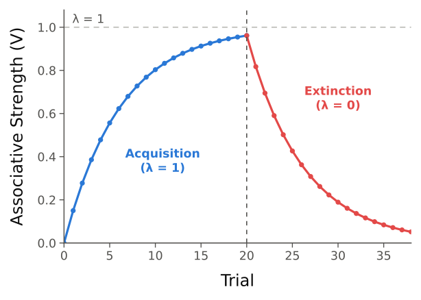
Figure: With $\alpha\beta = 0.15$ , associative strength $V$ rises toward the asymptote $\lambda = 1$ during acquisition (negatively accelerated, blue) and decays back toward zero once the US is removed and $\lambda = 0$ (extinction, red). The two phases mirror each other because the same prediction-error equation governs both; only the value of $\lambda$ changes.

Blocking Demonstration

Now we demonstrate blocking numerically. Suppose CS_A has been trained extensively in Phase 1:

After Phase 1: $V_A = 0.95$ (approximately at $\lambda = 1.0$ ).

In Phase 2, we present the compound CS_A + CS_B with the US. CS_B is a new stimulus with $V_B = 0$ , $\alpha_A = 0.3$ , and $\alpha_B = 0.3$ .

On each compound trial, the total associative strength is $V_A + V_B$ . The prediction error is computed against the compound total:

$\Delta V_A = \alpha_A \beta (\lambda - (V_A + V_B))$ $\Delta V_B = \alpha_B \beta (\lambda - (V_A + V_B))$

Phase 2 Trial	$V_A$	$V_B$	$V_A + V_B$	Prediction Error	$\Delta V_A$	$\Delta V_B$	New $V_A$	New $V_B$
1	0.950	0.000	0.950	0.050	0.008	0.008	0.958	0.008
2	0.958	0.008	0.966	0.034	0.005	0.005	0.963	0.013
3	0.963	0.013	0.976	0.024	0.004	0.004	0.967	0.017
4	0.967	0.017	0.984	0.016	0.002	0.002	0.969	0.019
5	0.969	0.019	0.988	0.012	0.002	0.002	0.971	0.021

After 5 compound trials, $V_B = 0.021$ which is essentially no change in conditioning. Compare this to what would happen if B had been conditioned alone from the start: after 5 solo trials, $V_B$ would be $1 - 0.85^5 = 0.556$ . The presence of the already-trained A has blocked learning about B by a factor of more than 25.

The blocking effect

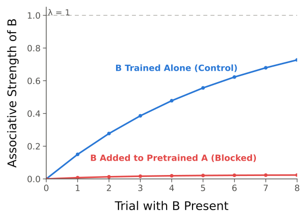
Figure: The blocking effect. Trained alone (control, blue), CS B acquires associative strength normally. Added to a compound with a pretrained CS A that already predicts the US (blocked, red), B gains almost nothing: A has already consumed the available prediction error, so $\lambda - (V_A + V_B) \approx 0$ and there is nothing left for B to learn. Contiguity between B and the US is identical in both conditions; only the prediction error differs.

Effect of Different Learning Rates

To illustrate the role of the rate parameters, compare three conditions with the same $\lambda = 1.0$ and $V_0 = 0$ :

Condition	$\alpha$	$\beta$	$\alpha\beta$	$V$ after 5 trials	$V$ after 10 trials	$V$ after 20 trials
Slow	0.1	0.2	0.02	0.096	0.183	0.332
Moderate	0.3	0.5	0.15	0.556	0.803	0.961
Fast	0.8	0.8	0.64	0.994	1.000	1.000

The shape of all three curves is the same---negatively accelerated exponential approach to $\lambda$ ---but the speed differs dramatically.

Assumptions and Limitations

The Rescorla-Wagner model, despite its enormous influence, rests on assumptions that constrain its applicability:

Trial-level processing: The model updates once per trial and does not represent within-trial timing of the CS, US, or expectation, even though real conditioning is exquisitely sensitive to the CS-US interval. Real-time models such as the temporal difference (TD) model and the Timing model of Gallistel and Gibbon (2000) address this.
Linear error correction: The change in $V$ is a linear function of the prediction error, with no mechanism for accelerating or decelerating learning based on the recent history of errors.
Fixed associability ( $\alpha$ ): CS salience does not change with experience, so the model cannot account for latent inhibition, learned irrelevance, or effects of prior discrimination training. This is the assumption Mackintosh (1975) and Pearce and Hall (1980) relaxed.
Summation of associative strengths: The model sums individual associative strengths rather than allowing configural processing, in which the compound AB is a distinct entity from A or B alone. Pearce's configural model (1987) addresses this.
No representation of time: All CS-US intervals are treated as equivalent and all intertrial intervals as irrelevant.
Symmetry of excitation and inhibition: The same equation governs both, though some evidence suggests they may follow different rules.
No memory or context effects: The model has no mechanism for spontaneous recovery, renewal, or reinstatement, phenomena suggesting that extinction creates a new, context-dependent inhibitory association rather than erasing the original.
US processing is constant: The parameter $\beta$ does not change with experience, ignoring habituation, motivation, and sensitization.

These limitations are not reasons to discard the model; they are the boundaries that define where it applies and where extensions are needed. Rescorla-Wagner remains the starting point for nearly all formal models of associative learning precisely because it is simple enough to understand clearly and powerful enough to generate surprising, testable predictions.

Connection to Empirical Behavior Science

The prediction-error signal formalized by Rescorla and Wagner became the conceptual foundation for temporal difference (TD) learning in artificial intelligence, which extends the trial-level update to moment-by-moment updating (Sutton & Barto, 1998); the later discovery that midbrain dopamine neurons encode a signal resembling the TD prediction error (Schultz, Dayan, & Montague, 1997) bridged behavioral learning theory, computational neuroscience, and AI.

Exercises for Reflection

The Rescorla-Wagner model predicts that if two separately trained excitatory CSs (A and B, each with $V \approx \lambda$ ) are presented together in compound with the US, both will lose associative strength. This is called overexpectation. Walk through the math: What is the prediction error on the first compound trial if $V_A = 0.95$ and $V_B = 0.95$ with $\lambda = 1.0$ ? What happens to $V_A$ and $V_B$ over the next few trials? Why is this prediction counterintuitive from a contiguity perspective?
Consider a clinical example: a client has a severe phobia of dogs (CS) associated with a traumatic bite (US). Describe the phobia in terms of associative strength. How would extinction (exposure therapy) work according to the Rescorla-Wagner model? What does the model predict about the rate of fear reduction across exposure sessions? What does the model fail to capture about real-world exposure therapy? (Think about spontaneous recovery, renewal, and reinstatement.)
Mackintosh's model allows $\alpha$ to change with experience, while the Rescorla-Wagner model holds $\alpha$ fixed. Design a thought experiment that would produce different predictions from the two models. Specify the training procedure, the test, and what each model predicts at test. (Hint: consider what happens when a CS has a long history of being irrelevant before it becomes a predictor.)

Key Readings

Required: Mackintosh (1975) proposed a theory of selective attention in associative learning in which the associability of a stimulus (i.e., its capacity to enter into new associations) changes with experience. Stimuli that are good predictors of outcomes gain associability; stimuli that are poor predictors lose it. This model addressed phenomena like learned irrelevance and the relative validity effect that the Rescorla-Wagner model could not easily explain, because Rescorla-Wagner treats the learning rate parameters as fixed constants. For the course, Mackintosh's model illustrates a critical modeling move: when a model fails on specific phenomena, the response is not to abandon it but to identify which assumption is too restrictive and relax it; in this case, making the learning rate itself a learnable quantity.

Matzel, Held, and Miller (1988) challenged the contiguity assumption that temporal ordering of CS and US is the primary determinant of conditioning. They presented evidence that simultaneous and backward CS-US pairings produce associations that are acquired but not always expressed in behavior, drawing a distinction between learning and performance that contiguity theory conflates. This paper matters for this week because it forces a confrontation with a fundamental modeling question: Does the Rescorla-Wagner equation describe learning itself, or does it describe the behavioral expression of learning? The answer has consequences for how we interpret parameters in associative learning models.

Supplemental: Rescorla and Wagner (1972) presented the original formal statement of the prediction-error learning rule that became the foundation of modern associative learning theory. Their model ( $\Delta V = \alpha\beta(\lambda - V)$ ) proposed that the change in associative strength on each trial is proportional to the discrepancy between what is expected and what occurs. This single equation unified a wide range of conditioning phenomena including acquisition, extinction, blocking, and conditioned inhibition under one quantitative framework. It is the canonical example of a formal model in behavior science and the starting point for everything covered this week.

Esber et al. (2025) revisited the Rescorla-Wagner model and argued that common textbook presentations misrepresent key aspects of the original formulation, particularly regarding the scope of the model's predictions and the role of its parameters. They clarified what the model actually claims versus what has been attributed to it through decades of secondary citation. This paper is a valuable corrective that demonstrates how formal models can drift from their original specification as they are transmitted through the literature which is a cautionary lesson for any modeler.

Stout and Miller (2007) formalized the comparator hypothesis as the Sometimes-Competing Retrieval (SOCR) model, which proposes that conditioned responding depends not on the absolute associative strength of a CS but on a comparison between the CS-US association and competing associations from the training context. Unlike Rescorla-Wagner, which locates all the action in the learning rule, SOCR places much of it in the retrieval and expression process. This paper broadens the week's perspective by showing that two models can agree on the learning mechanism yet diverge sharply on what controls the behavioral output---a distinction that has direct implications for how we design experiments to test between competing models.

Reading Guide

Mackintosh (1975)

What core problem in associative learning does Mackintosh's theory aim to address?
How does Mackintosh define "associability" in this context?
What role does attention play in his theory of learning?
What key idea distinguishes Mackintosh's theory from purely associative (e.g., Rescorla-Wagner) models?
According to the theory, what increases a stimulus's associability? What decreases it?
How does this model describe the adaptive capabilities of an organism within its environment?
What kind of empirical findings prompted Mackintosh to revise traditional associative learning theories?
How does Mackintosh's model explain the phenomenon of "blocking"?
How does this theory account for "learned irrelevance"?
Why is the notion of relative predictiveness central to this theory?
How does the model deal with compound stimuli (e.g., AX vs. BX)?
What are some criticisms or limitations of the model acknowledged by Mackintosh?
How might this theory relate to behavior analytic perspectives on discrimination learning?

Matzel, Held, & Miller (1988)

What central assumption of traditional contiguity theory do the authors challenge?
What is "simultaneous conditioning"? What is "backward conditioning"? How do these differ?
What evidence do the authors provide that contradicts the predictions of contiguity theory?
What is the distinction between the acquisition of an association and its behavioral expression?
How do the findings challenge the idea that temporal ordering determines association strength?
What broader implications does this work have for conditioning models in behavior science?

Connecting Forward

This week we saw how the Rescorla-Wagner model formalizes the way prediction errors across CS-US pairings build the associative strength a conditioned stimulus carries, and how Mackintosh's model makes attentional allocation itself a product of that history. Next week we turn to behavioral momentum theory, where the same kind of Pavlovian stimulus-reinforcer relationship, now operating at the level of the discriminative-stimulus context, determines how persistent behavior is when conditions change. Where Rescorla-Wagner tells us how associations form, behavioral momentum tells us how they make behavior resist change.

References

Gallistel, C. R., & Gibbon, J. (2000). Time, rate, and conditioning. Psychological Review, 107(2), 289--344. https://doi.org/10.1037/0033-295X.107.2.289

Kamin, L. J. (1969). Predictability, surprise, attention, and conditioning. In B. A. Campbell & R. M. Church (Eds.), Punishment and aversive behavior (pp. 279--296). Appleton-Century-Crofts.

Le Pelley, M. E. (2004). The role of associative history in models of associative learning: A selective review and a hybrid model. Quarterly Journal of Experimental Psychology Section B, 57(3), 193--243. https://doi.org/10.1080/02724990344000141

Mackintosh, N. J. (1975). A theory of attention: Variations in the associability of stimuli with reinforcement. Psychological Review, 82(4), 276--298. https://doi.org/10.1037/h0076778

Matzel, L. D., Held, F. P., & Miller, R. R. (1988). Information and expression of simultaneous and backward associations: Implications for contiguity theory. Learning and Motivation, 19(4), 317--344. https://doi.org/10.1016/0023-9690(88)90044-6

Miller, R. R., & Matzel, L. D. (1988). The comparator hypothesis: A response rule for the expression of associations. Psychology of Learning and Motivation, 22, 51--92. https://doi.org/10.1016/S0079-7421(08)60038-9

Pearce, J. M., & Hall, G. (1980). A model for Pavlovian learning: Variations in the effectiveness of conditioned but not of unconditioned stimuli. Psychological Review, 87(6), 532--552. https://doi.org/10.1037/0033-295X.87.6.532

Rescorla, R. A. (1969). Pavlovian conditioned inhibition. Psychological Bulletin, 72(2), 77--94. https://doi.org/10.1037/h0027760

Rescorla, R. A., & Wagner, A. R. (1972). A theory of Pavlovian conditioning: Variations in the effectiveness of reinforcement and nonreinforcement. In A. H. Black & W. F. Prokasy (Eds.), Classical conditioning II: Current research and theory (pp. 64--99). Appleton-Century-Crofts.

Schultz, W., Dayan, P., & Montague, P. R. (1997). A neural substrate of prediction and reward. Science, 275(5306), 1593--1599. https://doi.org/10.1126/science.275.5306.1593

Sutton, R. S., & Barto, A. G. (1981). Toward a modern theory of adaptive networks: Expectation and prediction. Psychological Review, 88(2), 135--170. https://doi.org/10.1037/0033-295X.88.2.135

Sutton, R. S., & Barto, A. G. (1998). Reinforcement learning: An introduction. MIT Press.

Key Takeaways

Prediction error drives learning. The Rescorla-Wagner model formalizes the idea that organisms learn when outcomes are surprising ( $\lambda - V \neq 0$ ) and stop learning when outcomes are fully predicted ( $\lambda - V = 0$ ). This was a revolutionary shift from contiguity-based accounts.
The Rescorla-Wagner equation: $\Delta V = \alpha\beta(\lambda - V)$ . A simple difference equation with three parameters: CS salience ( $\alpha$ ), US learning rate ( $\beta$ ), and asymptotic associative strength ( $\lambda$ ). Despite its simplicity, it generates a remarkably wide range of predictions.
Negatively accelerated learning curves emerge naturally from the model because prediction error shrinks as $V$ approaches $\lambda$ .
Blocking is explained by the summation of associative strengths: if one CS already predicts the US, there is no prediction error left for a second CS to capture. This showed that contiguity is not sufficient for learning and that informativeness matters.
Conditioned inhibition arises when a CS is paired with the absence of an expected US, driving $V$ below zero.
Overshadowing occurs when CSs of unequal salience compete for a shared prediction error, with the more salient CS gaining a larger share.
Overexpectation demonstrates that associative strength can decrease even when the US is present, if the compound prediction exceeds what the US supports.
Mackintosh's attention model extends the Rescorla-Wagner framework by allowing associability ( $\alpha$ ) to change with experience, accounting for learned irrelevance and other attentional phenomena.
Limitations of Rescorla-Wagner include trial-level processing, fixed $\alpha$ , no configural processing, no representation of time within trials, and no mechanism for context-dependent phenomena like spontaneous recovery. These limitations have motivated important extensions and alternative models.
The prediction error concept has had extraordinary reach, from animal learning theory to computational neuroscience (dopamine prediction error signals) to artificial intelligence (temporal difference learning).