Historical Models: Demand

Why This Topic Matters

Demand analysis asks how much of a commodity (reinforcer) an organism will consume as the price of that commodity changes, quantifying the relationship between price and consumption. The exponential demand equation developed by Hursh and Silberberg (2008) yields a small set of interpretable parameters, including demand intensity, essential value, and elasticity, that summarize an organism's consumption pattern. Its key advance over earlier power-function models was building normalization into the equation itself, so that parameters can be compared across commodities, individuals, and species.

---

Core Concepts

Demand and Consumption

Demand refers to the functional relationship between the price of a commodity and the amount consumed. Demand is not a single number, but a curve: as price increases, consumption typically decreases, and the shape of that decrease is informative. In behavior-analytic terms, consumption is the number of reinforcers obtained, and price is the response requirement per unit of reinforcer. The demand curve plots consumption as a function of price, typically after the organism has reached steady-state performance at each price.

Demand curves are typically plotted on double-logarithmic (log-log) axes for two reasons. First, price and consumption often span several orders of magnitude (e.g., FR 1 to FR 300, and 100 to 1 reinforcers), and log axes spread that range out instead of compressing the high-consumption data into one corner. Second, on log-log axes proportional changes are equal distances: a drop from 100 to 50 (50%) takes the same vertical distance as 10 to 5 (also 50%), making it easy to see whether the proportional decline is constant, accelerating, or decelerating. A key insight is that reinforcer value at a single price point can mislead: two reinforcers equally preferred when free may maintain very different behavior when the price is high.

It is also useful to distinguish between consumption and expenditure (or output). Consumption ($Q$) is the number of reinforcers obtained. Expenditure ($O$) is the total number of responses emitted to obtain those reinforcers. The relationship is:

$O = Q \times C$

where $C$ is the unit price. The two tell different stories: when demand is inelastic, consumption drops slowly but expenditure increases because the organism works harder per reinforcer; when demand is elastic, both decrease. The transition point, where expenditure is maximized, is $P_{max}$.

Unit Price

Unit price is defined as the ratio of the response requirement to the reinforcer magnitude:

$\text{Unit Price} = \frac{\text{Responses per Reinforcer}}{\text{Reinforcer Magnitude}}$

For a simple fixed-ratio (FR) schedule where each reinforcer delivery is identical, the unit price is simply the FR value. But the concept generalizes: an FR 20 delivering 2 pellets and an FR 10 delivering 1 pellet both have a unit price of 10 responses per pellet. The unit price equivalence assumption states that different combinations of response requirement and reinforcer magnitude producing the same unit price should produce the same consumption. This has substantial empirical support, particularly in closed economies, and lets researchers compare demand across schedule types and reinforcer magnitudes on a common scale. Note that unit price captures the ratio of effort to payoff but not all aspects of cost (e.g., the temporal cost of how long the schedule takes is not represented).

Elastic vs. Inelastic Demand

The rate at which consumption changes with price defines elasticity.

• Inelastic demand: Consumption changes relatively little as price increases; the organism keeps working despite rising costs. Essential commodities (food for a hungry organism, water for a thirsty one) tend to produce inelastic demand.

• Elastic demand: Consumption drops sharply as price increases; the organism quickly reduces or abandons consumption. Luxury commodities or those with readily available substitutes tend to produce elastic demand.

Most demand curves show mixed elasticity: inelastic at low prices (consumption is defended) and elastic at higher prices (consumption falls off). The price at which the curve transitions is $P_{max}$, the price that generates maximum total expenditure. Below $P_{max}$ the organism defends its consumption; above it, the rate of consumption decline outpaces the rate of price increase and total output (price $\times$ consumption) decreases.

More formally, at any given price demand is inelastic if a 1% increase in price produces less than a 1% decrease in consumption, and elastic if it produces more than a 1% decrease. At $P_{max}$ these rates are exactly equal (a 1% price increase produces a 1% consumption decrease): the point of unit elasticity.

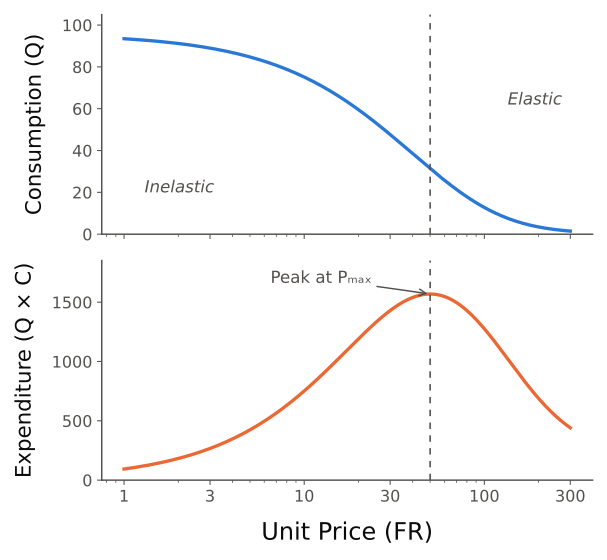
Figure: Why $P_{max}$ is the inelastic-to-elastic boundary. As unit price rises, consumption declines throughout (top), but total expenditure (the responses emitted, $Q \times C$) first rises and then falls, peaking at $P_{max}$ (bottom). Below $P_{max}$ demand is inelastic (the organism works harder to defend consumption, so expenditure climbs); above it demand is elastic (consumption falls faster than price rises, so expenditure drops).

The Exponential Demand Equation

Hursh and Silberberg (2008) proposed an exponential model of demand that has become the standard in behavioral economics:

$\log(Q) = \log(Q_0) + k \left( e^{-\alpha \cdot Q_0 \cdot C} - 1 \right)$

where:

• $Q$ is the consumption level (number of reinforcers obtained, or total amount consumed) at a given price.
• $Q_0$ is the demand intensity. That is, the level of consumption when price is zero (i.e., when the commodity is free).
• $\alpha$ (alpha) is the rate of decline in consumption as price increases. This parameter controls how quickly the demand curve bends downward.
• $k$ is the range constant, specifying the consumption range of the demand curve in log units, from $Q_0$ down to the lowest observed consumption level.
• $C$ is the cost or unit price

The equation operates in log-consumption space (often base 10). The term $e^{-\alpha \cdot Q_0 \cdot C}$ is an exponential decay function that drives consumption from its initial level ($Q_0$) toward zero as price increases, at a rate governed by $\alpha$.

A critical feature is that $\alpha$ and $Q_0$ appear together in the exponent as a product ($\alpha \cdot Q_0 \cdot C$). This is a normalized form. Consider water (500 ml per session when free) versus a flavored solution (50 ml when free): without normalization, water would show a larger absolute drop at any given price simply because its starting point is higher. Including $Q_0$ in the exponent rescales the price axis so that both commodities are evaluated in terms of proportional changes relative to their own baselines. This lets $\alpha$, and therefore essential value, serve as a rate-of-decline parameter comparable across commodities with different baseline consumption levels.

The subtracted 1 in $(e^{-\alpha \cdot Q_0 \cdot C} - 1)$ also plays a structural role. At $C = 0$ the exponential term equals 1, the parenthetical equals zero, and $\log(Q) = \log(Q_0)$: consumption equals demand intensity at zero price. As $C$ increases the exponential decreases toward 0, the parenthetical approaches $-1$, and $\log(Q)$ approaches $\log(Q_0) - k$. Thus $k$ sets the floor: the maximum number of log units consumption can decrease.

Essential Value

Essential value is defined as the reciprocal of $\alpha$:

$EV = \frac{1}{\alpha}$

This has been argued as the most important number that demand analysis produces. Essential value quantifies how resistant consumption is to price increases:

• A small $\alpha$ means consumption declines slowly with price. The commodity is hard to give up. Essential value ($1/\alpha$) is large.
• A large $\alpha$ means consumption declines quickly with price. The commodity is easy to give up. Essential value ($1/\alpha$) is small.

Essential value provides a single-number index of reinforcer efficacy that incorporates the entire demand curve, not just a single preference point. It answers the question: how much does this organism value this commodity, in the sense of being willing to pay increasing costs to maintain consumption? Its elegance is that a demand curve of potentially hundreds of data points collected over weeks can be distilled into one number that is easy to communicate and compare.

This simplicity comes at a cost. Essential value collapses the entire shape of the demand curve into one number, discarding information about $Q_0$, $k$, and the specific shape of the decline. Two commodities can have the same essential value but very different demand curves. For many purposes essential value alone is sufficient; for others, the full set of parameters is needed.

Q_0 --- Demand Intensity

$Q_0$ is the demand intensity: consumption when the commodity is free (price = zero). It reflects baseline preference in the absence of effort constraints, but is informative and incomplete. Two commodities can have identical $Q_0$ (equally consumed when free) but very different $\alpha$; the one with the smaller $\alpha$ (higher essential value) is the more potent reinforcer, because the organism defends its consumption as price increases.

This distinction highlights why free-access or FR 1 preference assessments can be misleading: they estimate $Q_0$ but tell us nothing about $\alpha$. In practice, $Q_0$ is usually estimated by extrapolation rather than direct measurement, because most designs do not include a truly free-access condition ($C = 0$); the lowest price tested (e.g., FR 1) approximates near-zero cost, and $Q_0$ is the model's estimate of consumption at zero cost. It is therefore partly a model-derived quantity rather than a pure observation, a subtle but important point when interpreting results.

Open vs. Closed Economies

The economic context in which demand is measured affects the results. In a closed economy, the experimental session is the organism's only source of the commodity (a rat that earns all of its food during the session). In an open economy, the organism has access to the commodity outside the session (a rat that receives supplemental food afterward regardless of how much it earned). Closed economies generally produce more inelastic demand, because the organism must work to obtain the commodity or go without. The practical consequence is that demand parameters estimated in open and closed economies are not directly comparable, so the economic context must be specified and parameters interpreted accordingly.

---

Applying the 8-Step Framework

Next, we walk through all 8 steps for modeling demand for food reinforcement in a food-deprived rat responding on ratio schedules in a closed economy.

Step 1: Identify All Environmental and Behavioral Components of the Phenomenon

A food-deprived rat is placed in an operant chamber with a lever that produces food pellets. Across conditions, the response requirement (FR value) changes: FR 1, FR 3, FR 10, FR 30, FR 100, FR 300, and so on, each maintained until responding is stable. At low FR values the rat consumes many pellets; as the FR increases it consumes fewer; at very high FR values it consumes very few or none. We want to model this entire relationship between price (FR value) and consumption (pellets earned), an orderly decline observed across species and commodities.

The demand equation does not model within-session dynamics (post-reinforcement pauses, bout structure). It takes the summary measure (total pellets earned per session), compresses each session into a single data point (consumption at that price), and asks what mathematical function describes how those points change across prices.

Step 2: Define the Behavioral Principles, Processes, and Intended Scope of the Model

We are modeling steady-state consumption as a function of unit price for a single commodity (food) in a single rat under a closed economy. The dependent variable is reinforcers obtained per session ($Q$); the independent variable is unit price ($C$), operationalized as the FR value (since reinforcer magnitude is constant, unit price equals FR value). We are not modeling:

• Within-session dynamics: How the rat distributes responding across the session (post-reinforcement pauses, bout structure).
• Transition effects: How behavior changes when the FR value shifts between conditions.
• Alternative reinforcement: The rat has no access to other commodities during the session.
• Individual differences: We model one rat's data at a time; group-level models require additional assumptions about parameter distributions across subjects.

Step 3: Write Down the Behavioral Principles, Known Quantitative Laws, and Functional Relationships

The candidate quantitative law is the Hursh-Silberberg exponential demand equation:

$\log(Q) = \log(Q_0) + k \left( e^{-\alpha \cdot Q_0 \cdot C} - 1 \right)$

This equation emerges from the behavioral-economic principle that consumption is governed by the interaction of the organism's valuation of the commodity and the cost of obtaining it. It replaces earlier power-function models, whose parameters were difficult to compare across commodities and species, by normalizing the rate parameter with respect to baseline consumption.

Step 4: State All Simplifying Assumptions Explicitly

1. Steady state: The organism has reached stable performance at each price point before consumption is measured.
2. Single commodity: Only one reinforcer is available. There are no substitutes within the session.
3. Closed economy: The session is the organism's sole source of food.
4. Constant motivation: Deprivation level (and thus the EO for food) is approximately constant across conditions.
5. Unit price equivalence: Price is fully captured by the FR value (reinforcer magnitude and lever effort are constant).
6. Shared $k$: The range constant $k$ is assumed equal across commodities and individuals within a dataset, allowing $\alpha$ values to be compared directly.
7. No income effects: The model ignores the organism's total response "budget"; at very high prices, income constraints may limit consumption independent of demand.
8. Log-linear relationship: The model operates in log-consumption space, treating proportional changes in consumption as the meaningful unit.

Each of these is a simplification of reality: the rat's MOs fluctuate, alternative reinforcement is never truly zero (the rat can groom, explore, sleep), and response capacity is finite. Stating the assumptions explicitly tells us exactly where the model might fail and lets us design tests of those boundaries.

Step 5: Write the Model Verbally, Then Express It Mathematically

Verbally: Consumption is a function of price. It is highest when price is at or near zero. As the FR requirement increases, the rat responds more to maintain contact with food, but past a certain point consumption decreases faster than the FR increases, and eventually contact with reinforcement stops altogether.

Mathematically: $\log_{10}(Q) = \log_{10}(Q_0) + k \left( e^{-\alpha \cdot Q_0 \cdot C} - 1 \right)$

The parameters are:

Symbol	Name	Interpretation	Units
$Q$	Consumption	Reinforcers obtained per session	Count
$Q_0$	Demand intensity	Consumption at zero price	Count
$\alpha$	Rate parameter	Rate at which consumption declines with price	1/(responses $\times$ count)
$k$	Range constant	Log-unit range of the demand curve	Dimensionless (log units)
$C$	Cost / Price	Response requirement per reinforcer (FR value)	Responses per reinforcer

The essential value is:

$EV = \frac{1}{\alpha}$

Step 6: Verify Dimensional Consistency

Dimensional analysis is a critical check: if the units do not work out, the equation is wrong regardless of how well it fits data. We verify two things: the exponent is dimensionless, and both sides have the same units. Consider the exponent $-\alpha \cdot Q_0 \cdot C$. For this to be dimensionless:

• $Q_0$ has units of reinforcers (count)
• $C$ has units of responses per reinforcer
• $Q_0 \cdot C$ has units of responses (count $\times$ responses/count = responses)
• $\alpha$ must therefore have units of 1/responses

The product $\alpha \cdot Q_0 \cdot C$ is then dimensionless (1/responses $\times$ responses = dimensionless). The exponential of a dimensionless number is dimensionless. Multiplying by $k$ (dimensionless, in log units) yields log units. Adding $\log(Q_0)$ (log units) to a quantity in log units yields log units. The left side, $\log(Q)$, is also in log units. Dimensions are consistent.

Step 7: Specify Starting Values and Constraints

• $Q_0 > 0$: Consumption at zero price must be positive (the organism consumes the commodity when it is free).
• $\alpha > 0$: The rate of decline must be positive (consumption decreases, not increases, with price).
• $k > 0$: The range constant must be positive. Common practice sets $k$ to a value shared across all curves in a dataset; Hursh and Silberberg (2008) suggested 2-4 for many behavioral datasets ($k = 3$ is common), or $k$ may be estimated from the data as $k = \log(Q_0) - \log(Q_{min})$, where $Q_{min}$ is the lowest observed non-zero consumption.
• $C \geq 0$: Price is non-negative. At $C = 0$, the equation yields $\log(Q) = \log(Q_0) + k(e^0 - 1) = \log(Q_0) + k(1-1) = \log(Q_0)$, confirming that consumption equals $Q_0$ at zero price.

These constraints follow from the behavioral interpretation: a negative $Q_0$ would mean negative consumption at zero price, and a negative $\alpha$ would mean consumption increases with price, contradicting the definition of demand. They thus guide fitting (bounding the search space) and interpretation (flagging implausible estimates as fitting failures).

For curve fitting, reasonable starting values might be:

• $Q_0$: Set to the observed consumption at the lowest price
• $\alpha$: Start with a small value such as $0.001$
• $k$: Fix at 3, or estimate from the data range

Step 8: Check the Math, Test Against Data, and Derive Predictions

Verify (boundary conditions):

• At $C = 0$: $\log(Q) = \log(Q_0) + k(e^0 - 1) = \log(Q_0) + 0 = \log(Q_0)$. So $Q = Q_0$. Correct: at zero price, consumption equals demand intensity.
• As $C \to \infty$: $e^{-\alpha \cdot Q_0 \cdot C} \to 0$, so $\log(Q) \to \log(Q_0) + k(0 - 1) = \log(Q_0) - k$. This means the minimum predicted consumption is $Q_0 \cdot 10^{-k}$. If $Q_0 = 100$ and $k = 3$, the minimum consumption is $100 \cdot 10^{-3} = 0.1$ reinforcers. In practice, consumption will hit zero before this asymptote.

Validate: Fit the equation to each rat's data using nonlinear least-squares regression on the log-transformed consumption values. Assess goodness of fit via $R^2$ and MAE, and examine residual plots for systematic deviations (a consistent over- or under-estimation pattern suggests the exponential form does not capture the curvature and motivates an alternative model). Typical $R^2$ values range from 0.85 to 0.99 in well-controlled studies.

Solve / Predict: Given estimated $Q_0$ and $\alpha$ (with $k$ fixed or estimated), predict consumption at any new price, compute essential value as $1/\alpha$, and compute $P_{max}$, the price at which behavioral output (total responses $= Q \times C$) is maximized. Setting $dO/dC = 0$ shows this occurs at the price of unit elasticity, where the price elasticity of demand equals $-1$ (the boundary between inelastic and elastic demand). For the exponential model this condition has no closed-form solution and is found numerically (we do so in the worked example below).

---

Worked Example

The Scenario

A food-deprived rat responds for 45-mg food pellets in a closed economy. Sessions last 24 hours, and the lever is the rat's only source of food. The experimenter varies the FR value across conditions, running each for 10 sessions and taking the mean of the last 5 (after stability) as the data point for that price.

Data

Steady-state consumption at each price is:

FR Value ($C$)	Pellets Earned ($Q$)	$\log_{10} Q$
1	90	1.954
3	85	1.929
10	70	1.845
30	40	1.602
60	18	1.255
100	6	0.778
300	1	0.000

Notice that consumption does not decline linearly: it drops slowly at first (about 22% from FR 1 to FR 10, 90 to 70) and then rapidly (85% from FR 30 to FR 100, 40 to 6). This accelerating decline is the hallmark of a demand curve transitioning from inelastic to elastic. The total responses (price $\times$ consumption) at each price are 90, 255, 700, 1200, 1080, 600, 300, peaking around FR 30 ($1{,}200$ responses) in these discrete data --- a first hint at where $P_{max}$ lies, which we compute from the fitted model below.

Fitting the Model

We fit the exponential demand equation:

$\log_{10}(Q) = \log_{10}(Q_0) + k \left( e^{-\alpha \cdot Q_0 \cdot C} - 1 \right)$

We fix $k = 2.5$ (estimated from the data range: $\log_{10}(90) - \log_{10}(1) \approx 1.95$, rounded up for headroom) and estimate $Q_0$ and $\alpha$ using nonlinear least-squares regression.

Step 1: Initial values.

• $Q_0 = 95$ (slightly above the highest observed consumption, since the lowest price tested is FR 1, not FR 0)
• $\alpha = 0.0001$ (a small starting value)

Step 2: Fit the model.

Using nonlinear regression (e.g., Python's scipy.optimize.curve_fit or R's nls), we minimize the sum of squared residuals between the observed $\log_{10}(Q)$ values and the predicted values, iteratively adjusting $Q_0$ and $\alpha$. After optimization, we obtain the best-fitting parameter estimates:

• $Q_0 = 96.2$
• $\alpha = 0.000328$
• $k = 2.5$ (fixed)

Step 3: Compute predicted values.

Using the original parameters, we generate predicted consumption at each price:

$C$	Observed $\log Q$	$-\alpha \cdot Q_0 \cdot C$	$e^{-\alpha \cdot Q_0 \cdot C}$	Predicted $\log Q$
1	1.954	$-0.0316$	0.969	1.906
3	1.929	$-0.0947$	0.910	1.759
10	1.845	$-0.3157$	0.729	1.306
30	1.602	$-0.9472$	0.388	0.454
60	1.255	$-1.8944$	0.150	$-0.129$
100	0.778	$-3.1573$	0.043	$-0.910$
300	0.000	$-9.4718$	0.000	$-1.517$

Note: the predicted values above use the initial parameter estimates, not the optimized ones. Real curve fitting iterates across all data points simultaneously, adjusting both $Q_0$ and $\alpha$ to minimize total error. After full nonlinear least-squares optimization, suppose the best-fitting parameters are:

• $Q_0 = 95.8$
• $\alpha = 0.000045$
• $k = 2.5$ (fixed)

Recomputing predicted values with these optimized parameters:

$C$	Observed $\log Q$	Predicted $\log Q$	Residual
1	1.954	1.971	$-0.017$
3	1.929	1.949	$-0.020$
10	1.845	1.873	$-0.028$
30	1.602	1.656	$-0.054$
60	1.255	1.224	0.031
100	0.778	0.727	0.051
300	0.000	$-0.340$	0.340

The residuals are now much smaller, and the model captures the shape of the decline well. The sum of squared residuals is $SSR = 0.017 + 0.020^2 + 0.028^2 + 0.054^2 + 0.031^2 + 0.051^2 + 0.340^2 \approx 0.124$. The $R^2$ value (computed against the total variance in $\log(Q)$) would be approximately 0.96, indicating an excellent fit.

The largest residual occurs at FR 300 ($0.340$ log units). This is common: at very high prices, consumption is near zero and highly variable, making precise prediction difficult. The model predicts slightly negative log-consumption (fractional pellets), which reflects the asymptotic floor of the curve; in practice, a predicted value below some threshold (e.g., less than 1 reinforcer) is interpreted as effective cessation of consumption. The residuals are small and show no strong systematic pattern, suggesting the exponential model is appropriate for these data.

Computing Essential Value

With our optimized $\alpha = 0.000045$:

$EV = \frac{1}{\alpha} = \frac{1}{0.000045} \approx 22{,}222$

This large essential value indicates that food, for this rat in a closed economy, is extremely highly valued: the rat defends its consumption vigorously as price increases. For comparison, if a saccharin solution tested in the same rat yielded $\alpha = 0.0035$, then:

$EV_{saccharin} = \frac{1}{0.0035} \approx 286$

Food ($EV \approx 22{,}222$) has roughly 78 times the essential value of saccharin ($EV \approx 286$), reducing the entire demand curve to a single number that supports direct comparison. Note that essential value is always relative to the conditions under which it was measured; it is a property of the organism-commodity-context system, not of the commodity alone.

Computing $P_{max}$

$P_{max}$ is the price at which total behavioral output ($O = Q \times C$) is maximized. Taking the derivative of $O$ and setting it to zero shows this happens at the price of unit elasticity, where the price elasticity of demand equals $-1$. For the exponential model this condition has no closed-form solution, so we solve it numerically. For our estimates ($Q_0 = 95.8$, $\alpha = 0.000045$, $k = 2.5$), the elasticity reaches $-1$ at:

$P_{max} \approx 50 \text{ responses per reinforcer (FR 50)}$

This means the rat's total behavioral output is maximized at approximately FR 50. Below this price demand is inelastic (increasing the FR increases total responding as the organism defends its consumption); above it demand is elastic (increasing the FR decreases total responding).

Two cautions are worth noting. First, a shortcut sometimes quoted for $P_{max}$, namely $0.368/(\alpha \cdot Q_0 \cdot k) \approx 34$, is only a rough approximation and understates the true value here: at FR 34 the elasticity is still about $-0.73$, so responding has not yet peaked. Always check such an approximation against the actual elasticity or the expenditure curve. Second, the fitted $P_{max}$ (FR 50) sits to the right of the raw data's expenditure peak (near FR 30, from the $1{,}200$-response condition). A fitted curve need not peak exactly where the sampled points do, and the gap is a useful cue to inspect how well the model captures the region around the peak.

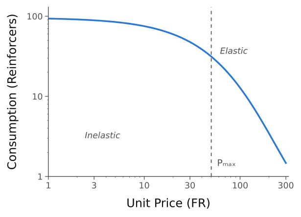
Figure: The fitted demand curve ($Q_0 = 95.8$, $\alpha = 0.000045$, $k = 2.5$) on double-logarithmic axes. Consumption is defended at low prices (the flat, inelastic region) and falls off steeply once price passes $P_{max}$, the unit-elasticity price (the elastic region). The parameter $\alpha$ controls how sharply the curve bends; its reciprocal is essential value.

Interpreting the Full Fit

Stepping back, the full analysis tells us the following about this rat's relationship with food under closed-economy conditions:

1. When food is free (or nearly free), the rat consumes about 96 pellets per session ($Q_0 = 95.8$): the baseline level of consumption without effort constraints, reflecting appetite and palatability.

2. The rat defends its food consumption vigorously as price increases ($\alpha = 0.000045$, $EV = 22{,}222$). The very small $\alpha$ means the demand curve bends slowly and the rat keeps working for food even at high FR values.

3. Maximum behavioral output occurs around FR 50 ($P_{max} \approx 50$, the unit-elasticity price). Below this price the rat compensates for price increases by responding more; above it, consumption declines faster than price increases and total responding decreases.

4. Even at very high prices, the rat does not fully abandon food (consumption at FR 300 is 1 pellet, not zero), characteristic of a highly essential commodity in a closed economy.

5. The demand curve fits the data well ($R^2 \approx 0.96$), indicating that the exponential model captures the overall shape of the price-consumption relationship.

This parameter-based interpretation is the payoff of the modeling enterprise. Rather than describing the data informally ("the rat responded less at higher FRs"), we can make precise, quantitative statements about demand intensity, essential value, and the transition between inelastic and elastic demand.

---

Assumptions and Limitations

The exponential demand equation rests on several assumptions that constrain its appropriate use:

• Steady-state behavior: Each data point must come from a condition in which the organism has reached stable performance; transitional data will not reflect true demand.
• Single commodity: The standard equation models one commodity in isolation. If substitutes are available, more complex models (e.g., cross-price demand) are required.
• No income effects: The model ignores total response capacity. At very high prices, an organism may fail to earn reinforcers because it physically cannot emit enough responses, not because it does not value them.
• Unit price equivalence: Only the ratio of responses to reinforcer magnitude is assumed to matter, not the specific combination. This holds reasonably well but can break down with very large or very small reinforcer magnitudes.
• Closed vs. open economy: Parameters are highly sensitive to economic context (open economies show higher $\alpha$, lower essential value), so comparing essential values across studies requires matching on context.
• The $k$ constant: Fixing the shared range constant $k$ allows $\alpha$ to be compared, but if $k$ genuinely differs, fixing it can distort $\alpha$ estimates.
• Log transformation and zeros: Because the model operates in log space, zero consumption is undefined ($\log 0 = -\infty$); handling this (adding a small constant, omitting zeros, or alternative formulations) introduces bias.
• Within-session dynamics and topography: The model predicts total consumption but says nothing about within-session response patterns, and parameter values are specific to the organism, commodity, and response form.
• Temporal discounting interactions: The equation does not account for delay between response and reinforcer; where delivery is delayed, effective value is discounted, and this demand-discounting interaction is an active area of development.

These limitations are not a reason to avoid the model; rather, they are a reason to use it carefully and interpret results within the boundaries the assumptions define.

---

Connection to Empirical Behavior Science

A key strength of the equation is its translational reach: the same parameters ($Q_0$, $\alpha$, essential value, $P_{max}$) apply across species, commodities, and settings, from rat lever pressing for food or drugs, to token-economy backup reinforcers, to human hypothetical purchase tasks. Because essential value is normalized, results from these very different preparations can be placed on a common quantitative scale.

---

Exercises for Reflection

1. Computing and comparing essential value. A researcher fits the exponential demand equation to consumption data for two drugs---Drug A and Drug B---in the same group of rats. Drug A yields $\alpha = 0.00025$ and Drug B yields $\alpha = 0.0082$. Both drugs have $Q_0 = 40$ infusions and $k = 3.0$.

   • Compute the essential value for each drug.
   • Which drug is the more potent reinforcer according to demand analysis?
   • Compute $P_{max}$ for each drug. At what FR value does behavioral output peak for each?
   • What behavioral pattern would you expect to see at high FR values (e.g., FR 200) for each drug? Describe the difference in concrete terms: what would the rats be doing differently?

2. Testing unit price equivalence. Design a hypothetical experiment to test whether an FR 20 schedule with 2-pellet reinforcers produces the same consumption as an FR 10 schedule with 1-pellet reinforcers. Specify the species, commodity, economic context, number of conditions, and stability criterion. What result would support the assumption, and what would challenge it? If it is violated, what are the consequences for interpreting demand curves that combine different schedule-magnitude combinations?

3. The role of $k$. The $k$ parameter is a "range constant" fixed across conditions in a dataset. Why might fixing it be problematic, and when might $k$ genuinely differ between commodities or individuals? If $k$ differs but is forced to be equal, how would this distort the estimated $\alpha$ values? Consider one commodity whose consumption ranges from 100 to 1 (a 2-log-unit range) and another from 100 to 0.01 (a 4-log-unit range): what happens if you fix $k = 3$ for both?

---

Alternative and Extended Models

The Hursh-Silberberg exponential form is one of several demand models. Its predecessor, the simple power function ($\log Q = \log a + b \cdot \log C$), has a constant slope $b$ and so predicts the same proportional decline at every price, missing the inelastic-to-elastic transition, and its parameters are not normalized for baseline consumption. The exponentiated demand equation (Koffarnus, Franck, Stein, & Bickel, 2015), $Q = Q_0 \cdot 10^{k(e^{-\alpha \cdot Q_0 \cdot C} - 1)}$, is the antilog of the standard equation and is preferred by some because it operates on consumption directly, accommodating zero values. Further extensions handle multiple commodities (cross-price demand) and integrate demand with delay discounting. All of these are descriptive models: they characterize the shape of the price-consumption relationship but do not specify the behavioral processes that generate it.

---

Key Readings

Required:

Hursh and Silberberg (2008) introduced the exponential demand equation and the concept of essential value as a normalized metric of reinforcer efficacy. Their model solved a long-standing problem in behavioral economics: earlier demand models used power functions whose parameters were not comparable across commodities or species. By building normalization into the equation itself through the $Q_0$ term in the exponent, Hursh and Silberberg created a framework in which the single parameter $\alpha$ (and its inverse, essential value) provides a universal index of how rapidly consumption declines as price increases. This paper is the mathematical backbone of the week and exemplifies how thoughtful model design can transform a descriptive tool into a translational one.

Francisco, Madden, and Borrero (2009) provided a primer on behavioral economics for applied behavior analysts, explaining core concepts such as demand, elasticity, unit price, open versus closed economies, and substitution in accessible language. They demonstrated how these concepts can inform the design of reinforcement-based interventions, token economies, and preference assessments. This paper bridges the gap between the formal demand models and clinical practice, showing that the quantitative framework is not an abstraction but a practical tool for understanding why clients consume some reinforcers vigorously and abandon others when the price rises.

Supplemental:

Hursh, Madden, Spiga, DeLeon, and Francisco (2013) reviewed the translational applications of the exponential demand model across substance abuse research, developmental disabilities, and health behavior. They argued that demand analysis provides a common quantitative language for comparing reinforcer value across populations and settings, making it one of the most portable tools in behavioral economics. This paper extends the week's core content by demonstrating the range of applied domains where the exponential demand equation has proven useful and reinforcing the course theme that formal models gain their greatest value when they travel across contexts.

---

Reading Guide

Hursh & Silberberg (2008)

• According to these authors, what are the 5 ways response strength has been defined historically? What are the benefits and drawbacks of each?
• What is the exponential demand equation proposed by Hursh & Silberberg (2008)?
• What does the parameter $Q_0$ represent?
• What does the parameter $\alpha$ (alpha) represent?
• What is "essential value," and how is it defined in the paper?
• What is the role of the parameter $k$?
• What theoretical advantage does the exponential model provide?
• Why is essential value considered a better reinforcer metric than $Q_0$ or break point?
• What is the general shape of the demand curve predicted by the exponential model?
• How does the model allow comparisons across reinforcers?
• What kind of reinforcers were used to validate the model?
• How did the exponential model perform in terms of data fit?
• How is essential value different from matching or discounting parameters?
• What is meant by "reinforcer magnitude" and how does it differ from essential value?
• What does the model predict about the effect of increasing reinforcer magnitude on $Q_0$ and $\alpha$?
• What is a potential limitation or caution in interpreting essential value?

Francisco, Madden, & Borrero (2009)

• What is behavioral economics and how does it differ from traditional economics?
• What is the primary dependent variable in behavioral economics?
• Define "demand" in the context of behavioral economics.
• What does it mean for demand to be "elastic" or "inelastic"?
• What is a demand curve and what does it depict?
• How is "price" typically operationalized in behavioral economics?
• What is "unit price" and why is it useful?
• How can behavioral economics inform drug abuse research?
• What is a "closed economy" vs. an "open economy"?
• How does economy type (open vs. closed) affect demand?
• What is "income" in behavioral economic terms?
• What is substitution in the context of behavioral economics?
• How might behavioral economics help in designing interventions?
• What is a practical takeaway for clinicians from this primer?

---

References

Francisco, M. T., Madden, G. J., & Borrero, J. C. (2009). Behavioral economics: Principles, procedures, and utility for applied behavior analysis. The Behavior Analyst Today, 10(2), 277--294. https://doi.org/10.1037/h0100671

Hursh, S. R. (1980). Economic concepts for the analysis of behavior. Journal of the Experimental Analysis of Behavior, 34(2), 219--238. https://doi.org/10.1901/jeab.1980.34-219

Hursh, S. R., & Silberberg, A. (2008). Economic demand and essential value. Psychological Review, 115(1), 186--198. https://doi.org/10.1037/0033-295X.115.1.186

Koffarnus, M. N., Franck, C. T., Stein, J. S., & Bickel, W. K. (2015). A modified exponential behavioral economic demand model to better describe consumption data. Experimental and Clinical Psychopharmacology, 23(6), 504--512. https://doi.org/10.1037/pha0000045

Nevin, J. A., & Grace, R. C. (2000). Behavioral momentum and the law of effect. Behavioral and Brain Sciences, 23(1), 73--90. https://doi.org/10.1017/S0140525X00002405

---

Key Takeaways

• Demand analysis quantifies the relationship between the price of a reinforcer and the amount consumed. It provides a richer picture of reinforcer value than preference assessments alone.

• Unit price ($C$) standardizes the cost of reinforcement as responses per unit of reinforcer, enabling comparison across schedule types and reinforcer magnitudes.

• The exponential demand equation --- $\log(Q) = \log(Q_0) + k(e^{-\alpha \cdot Q_0 \cdot C} - 1)$ --- is the standard model. It yields three key parameters: $Q_0$ (demand intensity), $\alpha$ (rate of decline), and $k$ (range constant).

• Essential value ($1/\alpha$) is the most important output of demand analysis. It indexes how resistant consumption is to price increases. Higher essential value means the reinforcer is harder to give up.

• $Q_0$ reflects baseline consumption when the reinforcer is free. It captures preference but not persistence.

• $P_{max}$ is the price that generates maximum behavioral output. Below $P_{max}$, demand is inelastic; above it, demand is elastic.

• Economic context matters: Closed economies produce more inelastic demand than open economies. Parameters are not comparable across economic contexts.

• Applications span drug self-administration, token economy design, and reinforcer assessment in clinical populations. The framework translates across species and settings.

• Limitations include the steady-state requirement, the single-commodity assumption, the treatment of zero consumption values, and the sensitivity of results to the fixed $k$ parameter.

• Historical context: The exponential demand equation (Hursh & Silberberg, 2008) solved the normalization problem that plagued earlier power-function models, enabling direct comparison of essential value across commodities and species.

• Translational utility: The same equation and parameters apply from rat lever pressing in the laboratory to human cigarette purchasing in survey studies, making demand analysis one of the most successfully translational frameworks in behavior science.