Historical Models: Matching and Discounting
Two hyperbolic models of how reinforcement parameters govern behavior
Why This Topic Matters
This week we study two hyperbolic models that turn qualitative intuitions about choice into precise quantitative predictions. The matching law describes how an organism allocates behavior across alternatives in proportion to the reinforcement each provides, and delay discounting describes the decline in subjective value of a reinforcer as the delay to its receipt increases. Both capture the same fundamental regularity, diminishing sensitivity to a schedule parameter (reinforcement rate in one case, delay in the other), and both are built on rectangular hyperbolas. We apply the 8-step modeling framework to matching and then extend the same logic to discounting.
Core Concepts: Matching
Choice as Behavior Allocation
From a behavior-analytic perspective, choice is not a mental event or a decision process hidden inside the organism. It is simply the allocation of behavior across available alternatives. This is the "molar view": rather than asking "Which key did the pigeon choose?" the question is "How did the pigeon distribute its behavior across the two keys over the session?" This framing turns choice into a continuous dependent variable that can be modeled with equations and predicted from environmental parameters. It also means choice is always happening: even in a single-schedule arrangement, the organism is choosing between the measured operant and all other available activities (grooming, exploring, resting). Recognizing that the single-schedule case is a special case of choice leads directly to quantitative predictions about response rate.
Herrnstein's Single-Alternative Matching
Herrnstein (1970) extended the matching law to the single-schedule case by reasoning as follows: if an organism always distributes behavior in proportion to relative reinforcement, then behavior on a single measured schedule depends on the reinforcement that schedule provides as well as on all other sources of reinforcement available in the environment. Unmeasured sources of reinforcement from alternative responses such as grooming, exploring, resting, and other activities are collectively called extraneous reinforcement and denoted .
The resulting model is known as Herrnstein's hyperbola:
where:
- is the observed response rate on the measured alternative (responses per minute)
- is the obtained reinforcement rate on the measured alternative (reinforcers per minute)
- is the asymptotic response rate: the maximum rate the organism would achieve if all reinforcement in the environment came from the measured alternative. It reflects motor capacity and motivational ceiling.
- is the extraneous reinforcement rate: the aggregate reinforcement from all unmeasured sources. It controls the curvature of the function.
The equation describes a rectangular hyperbola. When is small relative to , the term and the equation simplifies to , a straight line through the origin: responding increases approximately linearly with reinforcement. As grows large relative to , the term and : the function negatively accelerates and response rate approaches asymptotically. The half-maximum point occurs at , where . This gives a direct behavioral interpretation as the reinforcement rate at which responding reaches half its ceiling.
Why does the hyperbolic form arise? Consider the matching principle in its simplest form for the single-schedule case. The organism distributes its total behavioral output () across the measured operant and extraneous alternatives in proportion to the reinforcement each provides:
The fraction is the proportion of total reinforcement that comes from the measured alternative. The organism allocates the same proportion of its total behavioral output to that alternative. This is matching applied at the molar level, and it produces the hyperbola directly.
The Generalized Matching Equation (GME)
The original matching law states that relative response rate equals relative reinforcement rate. In practice, however, the match is rarely exact. Organisms sometimes undermatch (i.e., allocating behavior less extremely than reinforcement ratios would predict) or show a systematic bias toward one alternative (i.e., preference toward one alternative without correspondence to measured schedules of reinforcement). To accommodate these deviations, Baum (1974) proposed the generalized matching equation:
where:
- and are response rates (or time allocations) on alternatives 1 and 2
- and are reinforcement rates on alternatives 1 and 2
- is the sensitivity parameter (slope)
- is the bias parameter (the antilog of the intercept)
In its power-function form, the GME is written:
The log-ratio transformation linearizes this relationship, making it easy to fit with ordinary least-squares regression. A plot of against should yield a straight line with slope and intercept .
The key parameter is sensitivity (). When , the organism is strictly matching: the behavior ratio equals the reinforcement ratio. When (undermatching), behavior ratios are less extreme than reinforcement ratios (behavior is distributed more evenly than reinforcement predicts). When (overmatching), behavior ratios are more extreme, concentrating on the richer alternative beyond what the reinforcement differential predicts.
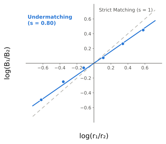
Figure: Sensitivity is the slope of the matching line. Plotting against linearizes the matching relationship; the slope is sensitivity and the intercept (not shown here) is bias. Real data typically show undermatching (): the fitted line (solid) is shallower than the strict-matching diagonal (dashed), so behavior is allocated less extremely than the reinforcement ratios alone would predict.
To understand why the log-ratio transformation is used, recall the basic algebra. Starting from the power-function form:
Take the logarithm (base 10) of both sides:
Apply the product rule of logarithms:
Apply the power rule of logarithms:
This is a linear equation of the form , where , , , and . The transformation converts a nonlinear relationship into a straight line fittable by ordinary least-squares regression. Base-10 logs are conventional (natural logs give the same slope and , only a rescaled intercept), so that a log ratio of 1.0 corresponds to a 10:1 ratio and 0.301 to a 2:1 ratio.
Undermatching and Overmatching
Undermatching () is the most commonly observed deviation from strict matching, with pigeon sensitivity values clustering around . It is driven mainly by low switching cost (frequent switching equalizes allocations; imposing a changeover delay pushes toward 1.0), poor discriminability between the alternatives, local rather than session-wide tracking of reinforcement, and the choice of response versus time measures. Overmatching () is rarer and tends to appear when switching is very costly or alternatives are highly discriminable. In applied settings, the sensitivity parameter tells you how well a client's behavior differentiates between better and worse reinforcement options: a client with low sensitivity may require larger reinforcement differentials to produce meaningful shifts in behavior allocation.
Bias
The bias parameter (, or equivalently as the intercept of the log-ratio regression) captures a systematic preference for one alternative that is not explained by the reinforcement rates. When (i.e., ), there is no bias and any preference is entirely attributable to observed differential reinforcement. When , the organism shows a systematic preference for alternative 1 even after reinforcement rates are accounted for. When , the preference favors alternative 2.
Bias can arise from differences between the alternatives that are unrelated to scheduled reinforcement rate: response topography or effort, spatial and positional side preferences, uncontrolled qualitative or magnitude differences in the reinforcers, stimulus features such as color, and reinforcement history. Notably, when reinforcer quality differs across alternatives, the bias parameter absorbs that difference, so researchers sometimes manipulate quality deliberately and use the GME as a measurement tool for it. In practice, bias is often small in well-controlled laboratory preparations (typically in pigeon concurrent VI-VI experiments), but its importance increases in applied settings where alternatives differ in many ways beyond reinforcement rate.
Applying the 8-Step Framework: Matching
We now will walk through all eight steps of the modeling framework for a concrete problem: modeling concurrent VI-VI schedule performance using the generalized matching equation.
Step 1: Get the Behavioral Phenomenon Clearly in Mind
A pigeon is placed in an operant chamber with two response keys (left and right). Each key is associated with an independent VI schedule of food reinforcement. In the condition of interest, the left key operates on a VI 60-s schedule (on average, one reinforcer becomes available every 60 seconds, yielding approximately 1 reinforcer per minute) and the right key operates on a VI 120-s schedule (on average, one reinforcer becomes available every 120 seconds, yielding approximately 0.5 reinforcers per minute). A 2-second changeover delay (COD) is in effect: after switching from one key to the other, the first peck on the new key cannot produce a reinforcer for 2 seconds.
The two VI schedules run independently and simultaneously; when a reinforcer is arranged by one schedule it waits ("holds") on that key until collected, and the COD penalizes rapid switching. After many sessions (typically 20--30 until response rates stabilize), the pigeon pecks the left key (VI 60-s) more than the right key (VI 120-s). But how much more, and how does this allocation change across other VI-VI combinations? The matching law provides the quantitative answer.
Step 2: Define the Behavioral Processes and Scope of the Model
We model the steady-state allocation of pecking across two concurrently available VI schedules. The model covers:
- Response allocation (pecks per minute on each key) at asymptotic performance
- The relationship between relative reinforcement rate and relative response rate across multiple conditions
- The degree to which the organism's behavior allocation tracks reinforcement ratios (sensitivity)
- Any systematic preference not attributable to reinforcement rates (bias)
The model does not cover:
- Acquisition of preference (how allocation changes during early exposure to new schedule values)
- Molecular response patterns (e.g., inter-response times, changeover patterns, visit durations)
- Within-session changes in preference (e.g., warm-up effects, satiation)
- Behavior during the changeover delay itself
- Effects of reinforcer magnitude, quality, or delay (these are held constant across alternatives)
- The mechanism by which matching arises (e.g., melioration, momentary maximizing)
These exclusions are deliberate: the GME is a molar, steady-state description whose utility lies in summarizing the endpoint of the choice process with two interpretable parameters, not in describing the process that generates matching.
Step 3: Identify the Behavioral Principles and Quantitative Laws
We invoke the matching principle: organisms distribute behavior across alternatives in proportion to the reinforcement obtained from those alternatives. The generalized form of this principle (Baum, 1974) allows for deviations from strict proportionality:
In log-ratio form:
This is the candidate quantitative law we will apply. It has been validated extensively across species (e.g., pigeons, rats, monkeys, humans), response types (e.g., key pecks, lever presses, time allocation, eye movements), and reinforcer types (e.g., food, water, brain stimulation, money, social interaction).
Step 4: State All Simplifying Assumptions
-
Steady state. Response rates have stabilized under each schedule-value pair, and we use only data from the last several sessions; the GME does not describe transitional behavior.
-
Independent schedules. Reinforcement arranged on one key is unaffected by responding on the other (except through the shared time constraint).
-
Single reinforcer type. Both alternatives deliver the same reinforcer, so allocation differences are due to reinforcement rate, not quality.
-
Changeover delay. A constant COD is in effect across conditions; its effects are absorbed into the sensitivity and bias parameters rather than modeled explicitly.
-
Molar account. The model describes session-wide aggregates rather than moment-to-moment dynamics.
-
Log-ratio linearity. The log behavior ratio is a linear function of the log reinforcement ratio, an empirical claim that holds well across concurrent VI-VI preparations but is an assumption nonetheless.
-
Constant motivation. Deprivation level is the same across conditions and stable within sessions.
-
No programmatic confounds. Schedule values are counterbalanced or randomized across keys so condition order does not bias the results.
Step 5: Write the Model Verbally, Then Mathematically
Verbal description: The log ratio of response rates on the two alternatives is a linear function of the log ratio of reinforcement rates on the two alternatives. The slope of this linear function captures how sensitive the organism is to changing reinforcement ratios. The intercept captures any systematic bias toward one alternative that is not due to reinforcement rate differences.
Mathematical expression:
In plain language: take the log of how much more the pigeon pecks one key than the other. This is predicted by a straight line whose input is the log of how much more reinforcement one key provides than the other. The slope tells you how steeply behavior tracks reinforcement. The intercept tells you whether the pigeon has an inherent preference for one side.
Equivalently, in the power-function form: the behavior ratio equals the reinforcement ratio raised to the power and multiplied by a bias constant . When and , this reduces to the original matching law: .
Step 6: Verify Dimensional Consistency
- : responses per minute divided by responses per minute = dimensionless.
- : reinforcers per minute divided by reinforcers per minute = dimensionless.
- : log of a dimensionless number = dimensionless.
- : log of a dimensionless number = dimensionless.
- : dimensionless (it is the slope relating two dimensionless log ratios).
- : dimensionless.
- : dimensionless + dimensionless = dimensionless.
Both sides of the equation are dimensionless. Units are consistent. Note that the log-ratio formulation has the feature of eliminating all physical units at the outset, so dimensional consistency is satisfied trivially. This is one of the practical advantages of the log-ratio approach.
Step 7: Specify Starting Values and Constraints
- : sensitivity must be positive; a negative value would mean more reinforcement produces less responding, contradicting the matching principle. Typical range , with common for response-rate measures and -- for time-allocation measures.
- (it is a ratio); (i.e., ) indicates no bias. Typical range in well-controlled pigeon experiments.
- The model applies to concurrent VI-VI schedules at steady state. Use at least three conditions (more is better) spanning a wide enough range of reinforcement ratios to give leverage for estimating the slope.
- Both and must exceed zero in every condition: exclusive preference makes the log ratio undefined, and that condition cannot be included.
Step 8: Check the Math, Test Against Data, and Derive Predictions
Verify. We check the model's predictions at informative boundary conditions:
- When : , so . With no bias (), : equal reinforcement produces equal responding.
- When (and ): , so the pigeon pecks key 1 more, increasingly so as the asymmetry grows.
- If and , the equation reduces to : strict matching. This confirms the GME nests the original matching law it was generalized from.
Validate. Fit the linear equation to data from our pigeon across multiple concurrent VI-VI conditions using ordinary least-squares regression. Compute and examine residuals for systematic patterns. In well-conducted experiments, values above 0.95 are typical, and residuals should show no systematic curvature.
Solve. For our specific example (VI 60-s vs. VI 120-s), if the pigeon obtains reinforcement rates close to the programmed rates:
- reinforcers/min (from the VI 60-s key)
- reinforcers/min (from the VI 120-s key)
If we have already estimated and from previous conditions:
The model predicts the pigeon will peck the VI 60-s key about 1.93 times as often as the VI 120-s key. Under strict matching (), the prediction would be a 2:1 ratio. The slightly lower predicted ratio (1.93:1) reflects the mild undermatching () partially offset by the small bias toward alternative 1 ().
If we further know that the pigeon's total response rate across both keys is about 60 pecks per minute, we can solve for the individual response rates:
These are concrete, testable predictions that can be compared to the pigeon's observed performance in the next session.
Worked Example: Matching
Dataset
A pigeon is exposed to five conditions of concurrent VI-VI schedules. In each condition, the pigeon responds on two keys for 25--30 sessions until response rates stabilize. The following data are obtained from the last five sessions of each condition (averaged):
| Condition | Left VI (s) | Right VI (s) | (reinf/min) | (reinf/min) | (resp/min) | (resp/min) |
|---|---|---|---|---|---|---|
| 1 | 30 | 120 | 1.85 | 0.47 | 52.3 | 12.1 |
| 2 | 60 | 60 | 0.94 | 0.91 | 28.7 | 25.9 |
| 3 | 120 | 30 | 0.46 | 1.88 | 11.8 | 49.7 |
| 4 | 45 | 90 | 1.28 | 0.63 | 40.1 | 18.6 |
| 5 | 90 | 45 | 0.64 | 1.31 | 19.2 | 38.4 |
Note that the reinforcement rates are obtained rates (what the pigeon actually contacted), which run slightly below programmed rates. The rich-vs-lean assignment alternates between left and right keys across conditions; this counterbalancing allows separation of sensitivity from side bias.
Step 1: Compute Ratios
For each condition, compute the response ratio and the reinforcement ratio :
| Condition | ||
|---|---|---|
| 1 | ||
| 2 | ||
| 3 | ||
| 4 | ||
| 5 |
Already we can see the matching pattern: when the reinforcement ratio favors the left key (Conditions 1, 2, 4), the response ratio also favors the left key, and vice versa (Conditions 3, 5). The response ratios are close to the reinforcement ratios but not identical. This is where the GME's sensitivity and bias parameters earn their keep.
Step 2: Compute Log Ratios
Transform to base-10 logarithms:
| Condition | ||
|---|---|---|
| 1 | ||
| 2 | ||
| 3 | ||
| 4 | ||
| 5 |
Note that Conditions 1 and 3 are approximate mirror images (the VI 30-s and VI 120-s schedules are swapped between keys). In log-ratio space they produce points approximately symmetric about the origin, exactly what should happen if the pigeon responds to relative reinforcement rather than to absolute features of a key location.
Step 3: Fit the Linear Equation
We fit the linear model using ordinary least-squares regression with as the predictor and as the outcome.
Compute the means:
Compute the deviations and cross-products:
| Condition | ||||
|---|---|---|---|---|
| 1 | ||||
| 2 | ||||
| 3 | ||||
| 4 | ||||
| 5 |
Compute the slope ():
Compute the intercept ():
Therefore:
The fitted equation is:
Step 4: Interpret the Parameters
Sensitivity: . This value is very close to 1.0, indicating that this pigeon is approximating strict matching: when the reinforcement ratio doubles, the behavior ratio slightly more than doubles. The 0.04 deviation toward overmatching is well within the sampling variability expected from a five-point regression, so we would not claim overmatching without more data and a formal test.
Bias: , or . The pigeon shows a very small bias toward the left key: even at approximately equal reinforcement rates (Condition 2), it pecks the left key slightly more (), responding about 4.5% more on the left key than the reinforcement ratio alone predicts. This could reflect a spatial preference or an idiosyncratic habit.
Step 5: Assess Goodness of Fit
The for this regression quantifies how well the GME accounts for the variance in behavior allocation across conditions.
Total sum of squares:
Regression sum of squares:
Residual sum of squares:
:
An of 0.999 indicates the GME accounts for essentially all the variance in behavior allocation across these five conditions, a level of fit typical for concurrent VI-VI data from well-trained pigeons.
Step 6: Generate a Prediction
Having fitted the model, we can predict the pigeon's behavior in a new, untested condition. Suppose we plan to expose the pigeon to concurrent VI 40-s VI 80-s. The expected reinforcement rates are approximately reinforcers/min and reinforcers/min.
The model predicts the pigeon will peck the left key about 2.15 times as often as the right key. This prediction can be tested by running the new condition and comparing the observed behavior ratio to 2.15.
From Matching to Discounting: The Same Mathematical Structure
The matching law and delay discounting are usually taught as separate topics, but they share a mathematical relationship that illuminates both. Consider the two core equations side by side:
Herrnstein's hyperbola (matching):
Mazur's hyperbola (discounting):
Both are rectangular hyperbolas. Both describe a dependent variable (response rate in one case, subjective value in the other) that changes as a function of an environmental parameter (reinforcement rate, delay). And both capture the same qualitative pattern: diminishing sensitivity. In Herrnstein's equation, each additional unit of reinforcement rate produces a smaller increment in response rate as grows; in Mazur's, each additional unit of delay produces a smaller decrement in subjective value as grows. The first units of the independent variable matter most.
This is not a coincidence. The matching law says organisms allocate behavior in proportion to relative reinforcement value. If the value of a reinforcer depends hyperbolically on its delay, then matching across alternatives that differ in delay produces the same systematic patterns seen in concurrent VI-VI schedules. In this sense the discounting function is a component of the matching framework: it specifies how delay transforms reinforcer value before that value enters the matching equation. The parallel extends to the parameters. In Herrnstein's hyperbola, controls how quickly response rate approaches its ceiling; in Mazur's, controls how quickly subjective value approaches its floor. Both are individual-difference variables.
The shared structure also contrasts with simpler alternatives: a linear model of matching would predict response rate increasing indefinitely (a physical impossibility), and an exponential model of discounting predicts constant proportional decline and unchanging preference between alternatives with constant relative delays. The practical payoff is that if you have mastered fitting, interpreting, and evaluating Herrnstein's hyperbola, you already have the toolkit for Mazur's. The 8-step framework and the diagnostic checks apply identically; only the behavioral domain changes.
Core Concepts: Discounting
Temporal Discounting
Temporal discounting refers to the decrease in subjective value of a reinforcer as the delay to its receipt increases (indexed by a reduction in the amount of behavior it will maintain). It refers specifically to the pure effect of delay, holding constant other reasons a delayed reward might be worth less (uncertainty that the promiser reneges, opportunity cost, inflation).
The key empirical tool for studying discounting is the indifference point: the amount of an immediate reward that a person (or animal) considers equivalent in value to a larger delayed reward. For example, if a participant is indifferent between $50 now and $100 in 6 months, then the indifference point at a 6-month delay is $50, so the subjective value of the delayed $100 is $50. Indifference points are measured with adjusting-amount, titrating (staircase), or fixed-choice-array procedures. By measuring indifference points at multiple delays, researchers fit a discount function to the data; the shape of that curve, linear, exponential, or something else, is the central question of discounting research.
Exponential Discounting
The exponential discounting model expresses subjective value as:
where:
- is the subjective value of the delayed reward
- is the amount (nominal value) of the delayed reward
- is the discount rate (a positive constant)
- is the delay to the reward
- is Euler's number (~2.718)
In plain language: the value of a reward decays by a constant proportion for each unit of time that passes. If a one-week delay reduces value by 10%, then a second week reduces the remaining value by another 10%, and so on. The decline is geometric, like radioactive decay.
To see why the proportional decline is constant, consider the ratio of values at two delays separated by one unit:
This ratio does not depend on . Whether you are comparing week 0 to week 1, or week 50 to week 51, the value drops by the same fraction . This is the defining property of exponential decay.
This constant-ratio property means exponential discounting produces consistent preferences: the relative preference between two rewards does not change as both move closer in time. This stationarity (or dynamic consistency) is why exponential discounting is considered normatively "rational" and is the standard model in neoclassical economics. The problem is that organisms routinely violate it: preferences reverse as options approach in time (we set an early alarm but hit snooze; we vow to quit drinking but stop for "just one beer"). Exponential discounting cannot account for these preference reversals.
Hyperbolic Discounting (Mazur)
Mazur's hyperbolic discounting model (Mazur, 1987) expresses subjective value as:
where , , , and are defined as above.
The critical difference from the exponential is the shape of the decay. The hyperbolic function declines steeply at short delays and then flattens out at longer delays. A reward delayed by one day from now loses much more value than a reward delayed by one additional day when it is already a year away. This is exactly what biological organisms do.
To see the difference in proportional decline, compute the same ratio as before:
This ratio does depend on . As increases, the ratio approaches 1, meaning each additional unit of delay produces a smaller proportional decline. The loss of value per unit delay is front-loaded: steep at first, increasingly shallow later. This is the mathematical signature of hyperbolic decay.
The hyperbolic form was not chosen arbitrarily: Mazur (1987) showed it provided a better quantitative fit than the exponential across a wide range of conditions, and it is now the standard descriptive model in the field. Note what the model is and is not. It is a descriptive model that tells us the shape of the discount function; it is not, by itself, an explanatory model of why the function is hyperbolic. Several mechanistic accounts have been proposed, but the descriptive model stands on its own empirical merits.
The k Parameter
The parameter in both the exponential and hyperbolic models is the discount rate. It controls how steeply value declines with delay.
- Higher : steeper discounting; value drops rapidly, corresponding to what is often called impulsive choice (preferring smaller-sooner reinforcers; though see Strickland & Johnson [2021] on the challenges with impulsivity as a construct).
- Lower : shallower discounting; value is well maintained across delays, corresponding to self-controlled choice (preferring larger-later reinforcers).
The parameter varies systematically across populations and conditions (for example, it is elevated in clinical populations such as those with substance use disorders). Two variations bear directly on the model's structure: differs within an individual across outcome types (health vs. money), so discounting is at least partly outcome-specific rather than a unitary trait; and for small amounts tends to be larger than for large amounts (the magnitude effect), which violates the assumption of an amount-independent .
Preference Reversals
Preference reversals are the signature prediction that distinguishes hyperbolic from exponential discounting. They occur when an organism's preference between two options switches as both options move closer in time.
For example, consider a choice between $50 available in 25 weeks and $100 available in 26 weeks. Many people prefer $100 in 26 weeks. Now move both options forward in time: $50 in 25 weeks versus $100 in 26 weeks becomes $50 now versus $100 in 1 week. As the smaller-sooner option approaches immediate availability, preference might switch to the smaller-sooner reward. This is a preference reversal.
How does the hyperbolic model account for this? Suppose the smaller-sooner reward is at delay , and the larger-later reward is at delay (the larger reward is always 1 week later than the smaller one). Using per week:
When (both far away):
- : Prefer the larger-later reward.
When (smaller reward available now):
- : Prefer the smaller-sooner reward.
Preference has reversed. Setting and solving for the crossing point gives weeks (about 6.3 days). When the smaller reward is more than ~0.9 weeks away, the larger-later reward is preferred. When the smaller reward is less than ~0.9 weeks away, preference switches to the smaller-sooner reward.
What happens with the exponential model? With the same parameters, the ratio is constant regardless of :
Because this ratio is always greater than 1 and does not depend on , the larger-later reward is preferred at every delay and preference never reverses. This is why preference reversals are the critical behavioral test: a qualitative prediction the hyperbolic model produces and the exponential cannot. Graphically, the reversal is the point where the two hyperbolic discount curves cross as both options approach in time.
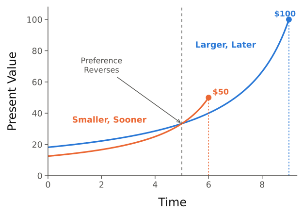
Figure: Why hyperbolic discounting produces preference reversals. Each curve is the present value of a reward as time advances toward its delivery (reward magnitudes marked at right). Far from both rewards, the larger-later reward ($100) is worth more and is preferred; as time approaches the smaller-sooner reward ($50), its steeply rising hyperbolic value overtakes the larger reward and preference reverses (dashed line). Exponential discounting, whose value ratio is constant, never produces this crossing.
Area Under the Curve (AUC)
Area under the curve (AUC) is a model-free measure of the degree of discounting (Myerson et al. 2001). Rather than fitting a parametric model, AUC treats the discount function as a set of empirical points connected by straight lines and computes the total area beneath that piecewise linear function.
The computation proceeds as follows:
- Normalize the x-axis (delay). Express each delay as a proportion of the maximum delay tested. The x-axis runs from 0 to 1.
- Normalize the y-axis (value). Express each indifference point as a proportion of the undiscounted amount (). The y-axis runs from 0 to 1.
- Add the origin point. At delay 0, value equals the full amount, so the point anchors the curve.
- Connect adjacent data points with straight lines, forming trapezoids between consecutive points and the x-axis.
- Sum the areas of the trapezoids. The area of each trapezoid is . The total is AUC.
AUC ranges from 0 to 1:
- AUC = 1: No discounting at all.
- AUC = 0: Complete discounting.
- Smaller AUC: Steeper discounting (more impulsive).
- Larger AUC: Shallower discounting (more self-controlled).
AUC makes no distributional assumptions, is not tied to any model form, and is straightforward to compute, but it discards information about the shape of the discount function, is sensitive to the number and spacing of delays tested, and yields no mechanistic parameter like . In practice, many researchers report both, using AUC for robust group comparisons and for mechanistic interpretation.
The Hyperboloid Model
The hyperboloid model (Green & Myerson, 2004; Myerson & Green, 1995) adds a scaling exponent to Mazur's hyperbola:
where is a free parameter that governs the overall scaling of the discounting process. When , the hyperboloid reduces to Mazur's hyperbolic model exactly. The hyperboloid provides a superior fit to many datasets, particularly human datasets.
The cost of the hyperboloid is an additional free parameter, which must be justified by a meaningful improvement in fit. Model comparison techniques (AIC, BIC, or cross-validation) are used to determine whether the improved fit warrants the added complexity.
Comparing the Three Discounting Models
| Feature | Exponential | Hyperbolic (Mazur) | Hyperboloid (Myerson et al.) |
|---|---|---|---|
| Equation | |||
| Free parameters | 1 () | 1 () | 2 (, ) |
| Proportional decline | Constant | Decreasing | Decreasing |
| Preference reversals | No | Yes | Yes |
| Empirical fit | Poor | Good | Best (in many cases) |
| Normative status | "Rational" standard | Descriptive standard | Extended descriptive |
| Special case | --- | Hyperboloid with | General form |
The progression from exponential to hyperbolic to hyperboloid illustrates a general principle in modeling: start simple, add complexity when the data demand it, and always ask whether the added complexity is justified by improved fit or new qualitative predictions.
Worked Example: Discounting
Following the same 8-step logic applied to matching above, we now fit Mazur's hyperbolic model to delay discounting data. Rather than repeating every step in full, we focus on the key elements: the equation, the fitting procedure, the interpretation of , and the comparison with the exponential model.
The Data
A participant makes choices between an immediate monetary reward and $100 available at each of seven delays. Using an adjusting amount procedure, we determine the indifference point at each delay:
| Delay (weeks) | Indifference Point ($) |
|---|---|
| 1 | 90.00 |
| 2 | 82.00 |
| 4 | 70.00 |
| 8 | 55.00 |
| 16 | 38.00 |
| 26 | 28.00 |
| 52 | 18.00 |
Notice the pattern before fitting any model. The drop from delay 1 to delay 2 (one additional week) is $8. The drop from delay 26 to delay 52 (26 additional weeks!) is $10. Despite the much larger increase in delay, the decrease in value is only slightly larger. This is the hallmark of hyperbolic, not exponential, decay.
Fitting the Hyperbolic Model
The model is . Rearranging to isolate from each data point: .
| Delay () | Observed | estimate |
|---|---|---|
| 1 | 90.00 | |
| 2 | 82.00 | |
| 4 | 70.00 | |
| 8 | 55.00 | |
| 16 | 38.00 | |
| 26 | 28.00 | |
| 52 | 18.00 |
The estimates cluster around per week. The consistency across delays is impressive and already indicates the hyperbolic model is a good description. Using , the predicted values and residuals are:
| Delay () | Observed | Predicted | Residual |
|---|---|---|---|
| 1 | 90.00 | 90.91 | |
| 2 | 82.00 | 83.33 | |
| 4 | 70.00 | 71.43 | |
| 8 | 55.00 | 55.56 | |
| 16 | 38.00 | 38.46 | |
| 26 | 28.00 | 27.78 | |
| 52 | 18.00 | 16.13 |
The ---the hyperbolic model accounts for 99.8% of the variance.
Interpreting k
The estimated per week tells us:
- The half-life of value is weeks. After 10 weeks of delay, this participant's subjective value drops to half its face value.
- This is a moderately steep discounter. If choosing between $50 now and $100 in 10 weeks, this participant would be approximately indifferent.
Comparing with the Exponential Model
Fitting reveals a diagnostic problem: the point-by-point estimates decline systematically from 0.105 at to 0.033 at . This declining pattern is the signature of data that are hyperbolic, not exponential. No single exponential can describe these data well.
Using the average exponential , the exponential model significantly underpredicts subjective value at long delays, predicting $2.24 at 52 weeks when the actual indifference point is $18.00. The exponential , compared to the hyperbolic's . The hyperbolic model fits roughly 59 times better by sum of squared residuals.
Computing AUC
Normalizing both axes (delay divided by 52, value divided by 100) and summing trapezoid areas yields: AUC = 0.362, indicating moderately steep discounting. AUC values below 0.50 generally reflect substantial discounting.
Applied Significance of Discounting
The value of the parameter connects the model to applied concerns: steep discounting (high ) is reliably elevated in clinical populations such as those with substance use disorders, ADHD, obesity, and problem gambling, which is why is often treated as a behavioral marker and intervention target. Several evidence-based interventions map directly onto the discount function, including contingency management (supplying a competing immediate reinforcer, note the relation to matching), episodic future thinking (reducing the perceived delay to a future outcome), and precommitment (locking in the larger-later preference before the preference-reversal point arrives).
Assumptions and Limitations of Discounting
Mazur's hyperbolic model rests on several simplifying assumptions:
- Single reinforcer. One delayed outcome is considered in isolation; interactions among multiple delayed outcomes are not captured.
- Stable preferences. is assumed fixed within a session, though in practice it shifts with motivating operations, competing schedules, stress, effort, and framing.
- Amount-independent . Larger amounts are actually discounted less steeply (the magnitude effect), one of the most reliable violations of the simple model.
- Time as the only dimension. Real intertemporal choices also involve uncertainty, effort, and opportunity cost, which the basic model collapses into delay alone.
- Static model. It describes the steady-state delay-value relationship and says nothing about how discounting develops or changes with intervention.
- Functional form. The hyperbolic is a good empirical description but is not derived from first principles.
- Nonsystematic data. Indifference points that do not decrease monotonically with delay violate the premise of discounting and suggest inattention.
As with the matching assumptions above, these are not flaws; rather, they are the explicit boundaries of the model, which tell us precisely what it claims and what it does not.
Key Readings
Matching:
Reed and Kaplan (2011) provided a practitioner-oriented tutorial on the matching law, demonstrating how to conduct and interpret matching analyses with applied behavioral data. They walked through the generalized matching equation, explained the meaning of the sensitivity and bias parameters, and showed how matching analyses can be used to evaluate reinforcement-based interventions. This paper grounds the matching law in practical application and makes the case that quantitative models of choice are not just for the basic laboratory---they are tools that practitioners can and should use to understand why clients allocate behavior the way they do.
McDowell (1989) identified two developments that reshaped matching theory after Herrnstein's original formulation: the extension to asymmetrical choice situations and the problem of undermatching. He argued that while bias (asymmetry) is a predictable and theoretically benign departure from strict matching, undermatching poses a genuine challenge to the theory because it suggests organisms are less sensitive to reinforcement ratios than the matching law predicts. This paper is essential for understanding that the matching law is not a settled empirical fact but an evolving quantitative framework, and it introduces the distinction between deviations that a model accommodates and deviations that demand revision.
Fisher and Mazur (1997) bridged basic and applied research on choice by reviewing how concurrent-schedule procedures and the matching law have been used to understand clinically significant behavior. They demonstrated that choice between appropriate and inappropriate behavior can be analyzed using the same quantitative framework that describes pigeon key pecking, and they reviewed applications including functional analysis and treatment evaluation. This paper connects the formal models of choice covered this week to the applied questions that motivate much of behavior analysis, showing that the matching law is not merely a laboratory curiosity but a quantitative tool for understanding and changing socially important behavior.
Discounting: Critchfield and Kollins (2001) made the case that temporal discounting---the decline in reinforcer value with delay---is not just a basic research phenomenon but a variable that underlies many socially important behaviors, including substance abuse, academic performance, and health-related decision making. They reviewed the empirical evidence linking steep discounting to impulsive behavior patterns and argued that the discounting framework provides a quantitative handle on problems that behavior analysts encounter daily. This paper establishes why discounting models matter beyond the laboratory and sets up the course theme that formal models gain their value when they connect to real-world behavioral phenomena.
Rachlin (2006) offered a theoretical treatment of discounting that clarified several conceptual issues, including the distinction between delay discounting and probability discounting, the relationship between the two, and the implications of hyperbolic versus exponential functional forms. He argued that the hyperbolic form is not merely a better empirical fit but reflects something fundamental about how organisms integrate information about delayed consequences. This paper deepens the theoretical understanding of the discounting models introduced this week and illustrates how careful attention to functional form---a core theme of the course---can yield insight into behavioral mechanism.
Odum et al. (2020) reviewed the literature on delay discounting across different outcome types---money, health, food, drugs---and asked whether discounting is a unitary process or whether different outcomes engage different valuation mechanisms. They presented a theoretical framework for understanding cross-commodity differences in discounting and discussed the implications for both basic theory and clinical application. This paper extends the week's models by raising the question of generality: does one discounting equation with one set of parameters describe all reinforcers, or must the model be adapted for different outcome domains?
Cox and Dallery (2018) examined how delay and probability combine to affect the subjective value of reinforcers in humans. They tested whether delay discounting and probability discounting operate independently or interact, finding that the combined effects of delay and probability are not simply additive. This paper contributes to the week's framework by pushing the boundaries of single-variable discounting models and demonstrating that real-world choices often involve simultaneous variation in multiple reinforcer dimensions---a complexity that simple hyperbolic models must eventually confront.
Reading Guide
Reed & Kaplan (2011)
- How do the authors define "choice" from a behavior analytic perspective?
- What is the matching law, and what does it predict?
- Describe how Herrnstein's original experiment with pigeons led to the matching law.
- How can relative response rates be used to infer preference?
- Why use ratios (B1/B2 and R1/R2) in matching analyses?
- How is matching observed in real-world behavior (e.g., classrooms, playgrounds)?
- What is the Generalized Matching Equation (GME), and how does it build on the original?
- What do the parameters b (bias) and s (sensitivity) represent in the GME?
- How can we interpret the slope and intercept of a matching line?
- What are common sources of bias in applied matching analyses?
- What kind of data would you need to conduct a matching analysis in practice?
- How do different reinforcer dimensions (rate, quality, effort, delay) affect matching outcomes?
- How might one use matching analyses to evaluate the effectiveness of intervention strategies?
- How can a practitioner use the bias parameter to tailor treatment?
- What are some limitations of matching law applications in applied contexts?
McDowell (1989)
- What is meant by "asymmetrical choice situations"?
- Why are most natural human choice situations considered asymmetrical?
- What mathematical form does McDowell discuss for asymmetrical choice?
- How does this power function differ from the original (linear) matching law?
- Why might a power function better describe human choice behavior?
- What does McDowell refer to by "indifferent responding"?
- Why does McDowell believe biased responding IS NOT a big deal for matching theory?
- Why does McDowell believe undermatching IS a big deal for matching theory?
Fisher & Mazur (1997)
- What is the primary focus of this article in terms of research synthesis?
- How do the authors define "choice responding"?
- What is the role of concurrent schedules in studying choice?
- What kinds of dependent variables are typically used in choice research?
- What are some of the reinforcer dimensions shown to influence choice responding?
- How have researchers used choice procedures to study problem behavior?
- How do Fisher and Mazur connect laboratory-based findings with applied intervention strategies?
- Why is it important to distinguish between molar and molecular analyses of behavior?
- How can quantitative modeling support individualized treatment planning?
Critchfield & Kollins (2001)
- What is temporal discounting?
- How does temporal discounting relate to self-control?
- How do the authors distinguish behavior analysis from cognitive models of choice?
- What does the parameter represent in Mazur's hyperbolic model?
- How well does Mazur's hyperbolic equation fit human discounting data?
- Why are hypothetical rewards used instead of real rewards in many studies?
- How do temporal discounting patterns differ across populations?
- How can delay sensitivity be functionally relevant for understanding ADHD?
- How might ABA practitioners apply discounting research to treatment planning?
Rachlin (2006)
- How does Rachlin define discounting in the context of behavioral choice?
- What is the difference between exponential and hyperbolic discounting?
- Why does Rachlin argue that hyperbolic discounting leads to preference reversals?
- How does Rachlin explain self-control in terms of temporal discounting?
- What role do commitment strategies play in self-control according to Rachlin?
- What is meant by "bundling" in Rachlin's theory of self-control?
- What is the key difference between molar and molecular views of self-control?
- What implications does Rachlin draw for public health and policy?
Odum et al. (2020)
- What does it mean to say discounting is "outcome-specific"?
- How does monetary discounting compare to discounting of other outcomes?
- What is the magnitude effect in delay discounting?
- What is the sign effect in discounting research?
- How do individual differences influence discounting?
- What implications do the findings have for intervention design?
Exercises for Reflection
-
Consider a clinical scenario in which a child engages in both appropriate play and disruptive behavior during a therapy session. If functional analysis data show that the child receives adult attention for disruptive behavior on average every 2 minutes and for appropriate play on average every 10 minutes, what does the matching law predict about the allocation of behavior? How would you change the reinforcement environment to shift the allocation toward appropriate play? Be specific about what reinforcement ratio you would target and why.
-
The sensitivity parameter is typically less than 1.0, indicating undermatching. In an applied context, why might undermatching actually be beneficial for the client? Consider what would happen if a client showed perfect matching () or overmatching () in an environment where reinforcement contingencies are imperfect or variable.
-
A participant shows an indifference point of $75 for $100 delayed by 4 weeks and an indifference point of $25 for $100 delayed by 52 weeks. Estimate from each data point using Mazur's equation. Are the two estimates similar? What would it mean if they were very different?
-
Exponential discounting predicts no preference reversals, yet preference reversals are commonly observed. Design a simple experiment (choice between a smaller-sooner and a larger-later reward at varying time horizons) that would test for preference reversals. Specify the amounts, the delays, and the expected pattern of choices under both exponential and hyperbolic discounting.
-
Both Herrnstein's hyperbola and Mazur's hyperbola are rectangular hyperbolas with a "half-life" parameter ( for matching, for discounting). Compare and contrast these two parameters. What does each one tell you about the organism? How would you use each one in an applied context---for example, to design a reinforcement-based intervention for a client?
References
Baum, W. M. (1974). On two types of deviation from the matching law: Bias and undermatching. Journal of the Experimental Analysis of Behavior, 22(1), 231--242. https://doi.org/10.1901/jeab.1974.22-231
Cox, D. J., & Dallery, J. (2018). Influence of second outcome on monetary discounting. Behavioural Processes, 153, 84--91. https://doi.org/10.1016/j.beproc.2018.05.012
Critchfield, T. S., & Kollins, S. H. (2001). Temporal discounting: Basic research and the analysis of socially important behavior. Journal of Applied Behavior Analysis, 34(1), 101--122. https://doi.org/10.1901/jaba.2001.34-101
Fisher, W. W., & Mazur, J. E. (1997). Basic and applied research on choice responding. Journal of Applied Behavior Analysis, 30(3), 387--410. https://doi.org/10.1901/jaba.1997.30-387
Herrnstein, R. J. (1961). Relative and absolute strength of response as a function of frequency of reinforcement. Journal of the Experimental Analysis of Behavior, 4(3), 267--272. https://doi.org/10.1901/jeab.1961.4-267
Herrnstein, R. J. (1970). On the law of effect. Journal of the Experimental Analysis of Behavior, 13(2), 243--266. https://doi.org/10.1901/jeab.1970.13-243
Mazur, J. E. (1987). An adjusting procedure for studying delayed reinforcement. In M. L. Commons, J. E. Mazur, J. A. Nevin, & H. Rachlin (Eds.), Quantitative analyses of behavior: Vol. 5. The effect of delay and of intervening events on reinforcement value (pp. 55--73). Erlbaum.
McDowell, J. J. (1989). Two modern developments in matching theory. The Behavior Analyst, 12(2), 153--166. https://doi.org/10.1007/BF03392492
Odum, A. L., Becker, R. J., Haynes, J. M., Galizio, A., Frye, C. C. J., Downey, H., Friedel, J. E., & Perez, D. M. (2020). Delay discounting of different outcomes: Review and theory. Journal of the Experimental Analysis of Behavior, 113(3), 657--679. https://doi.org/10.1002/jeab.589
Rachlin, H. (2006). Notes on discounting. Journal of the Experimental Analysis of Behavior, 85(3), 425--435. https://doi.org/10.1901/jeab.2006.85-05
Reed, D. D., & Kaplan, B. A. (2011). The matching law: A tutorial for practitioners. Behavior Analysis in Practice, 4(2), 15--24. https://doi.org/10.1007/BF03391780
Key Takeaways
-
Choice is behavior allocation. From a behavior-analytic perspective, choice is the measurable distribution of behavior across available alternatives, not a private mental event. This framing makes choice a continuous variable amenable to quantitative modeling.
-
The matching law states that the relative rate of responding on an alternative approximately equals the relative rate of reinforcement obtained from that alternative. First published by Herrnstein (1961) with pigeons on concurrent VI schedules, it was the first quantitative law of choice in behavior science.
-
Herrnstein's hyperbola, , extends matching to the single-schedule case by recognizing that all behavior occurs in a context of competing reinforcement sources. The parameter is the asymptotic response rate, and is the extraneous reinforcement rate.
-
The generalized matching equation (GME), , is the standard tool for analyzing concurrent-schedule data. Sensitivity () measures how precisely behavior tracks reinforcement ratios; bias () captures systematic preference unrelated to reinforcement rates.
-
Temporal discounting is the decline in subjective value of a reinforcer as the delay to its receipt increases. It is one of the most robust quantitative regularities in behavior science, observed across species, reinforcer types, and populations.
-
Hyperbolic discounting (, Mazur, 1987) assumes a decreasing proportional decline in reinforcer value. That is, steep at short delays, shallow at long delays. It often fits empirical data better than the exponential model () and correctly predicts preference reversals.
-
The matching and discounting hyperbolas share the same mathematical structure. Both are rectangular hyperbolas describing diminishing sensitivity to a schedule parameter. Herrnstein's and Mazur's both define a "half-life" that characterizes the system's sensitivity.
-
The parameter in discounting is the discount rate. Higher = steeper discounting = more "impulsive" choice. The half-life of value is .
-
Area under the curve (AUC) is a model-free measure of discounting, normalized from 0 to 1, that requires no distributional assumptions.
-
Clinical significance: The matching law informs functional analysis and treatment evaluation by quantifying the reinforcement contingencies governing behavior allocation. Steep discounting is reliably associated with substance abuse, ADHD, obesity, and gambling. Together, these models provide quantitative tools for assessment and intervention design.
-
Limitations: The GME is a molar, steady-state, two-alternative model. Mazur's hyperbola assumes stable, amount-independent discounting of a single outcome. Both models are descriptive, not mechanistic. These limitations define their scope and point toward the dynamic and computational models covered in later weeks.