Week 1: Introduction to Modeling in Behavior Science

Why This Topic Matters

Behavior science aspires to be a natural science of behavior, and natural sciences make quantitative predictions. They do this through models: formal representations of how processes work that can be tested against observation. The experimental analysis of behavior has produced impressive quantitative regularities (the matching law, delay discounting functions, demand curves). This week highlights how each of these are instances of a general modeling framework commong among all natural sciences.

Models matter because they force clarity. A verbal claim such as "reinforcement strengthens behavior" might be generally correct. However, it does not tell you by how much, under what conditions, or how the effect changes when parameters change. A mathematical model has to answer these questions explicitly. Models also matter because they are the bridge between basic findings and application. If you want to predict how a token economy will perform, or how changing the price of a commodity will alter consumption, you need a quantitative framework. Stated differently, precision in predictions requires a model, not just principles.

Understanding what models are and are not is equally important. A model is not reality. It is a deliberately simplified representation of some aspect of reality, constructed to predict, explain, or both. All models are wrong in the sense that they omit details. Useful models are wrong in ways that do not matter for the question at hand. The art of modeling lies in choosing what to leave out.

Abstraction is the modeler's primary tool. Abstraction involves identifying the features of a phenomenon that are essential for the question being asked and to discard the rest. A cumulative record abstracts away the topography of each response and retains only its time of occurrence. Response rate abstracts further, collapsing a stream of events into a single number. Every model involves choices about the level and type of abstraction, and those choices are made deliberately by the modeler.

Core Concepts

What Is a Model?

A model is a formal representation of a system or process. "Formal" means the representation is expressed in a language with explicit rules (e.g., mathematics, computer code, logic). The representation specifies the components of the system, the relationships among them, and the rules by which the system changes over time or across conditions.

Types of Models

Verbal models state claims in natural language. "Behavior is a function of its consequences" is a verbal model. Verbal models are useful starting points but are often imprecise in description and prediction and, therefore, difficult to test rigorously.

Mathematical models express claims as equations. $R = \frac{k \cdot r}{r + r_e}$ is a mathematical model (Herrnstein's hyperbola). The relationships are explicit, the parameters are defined, and predictions are quantitative.

Computational models implement processes as algorithms. Rather than writing a closed-form equation, a computational model specifies rules that are executed step by step. Much of machine learning and artificial intelligence falls in this category.

Simulation models are computational models run forward in time to generate synthetic data. They are especially useful when a system's behavior is too complex to solve analytically.

These categories overlap. A mathematical model can be implemented computationally; a simulation can be based on a mathematical model. The distinctions are more about emphasis as opposed to being rigid boundaries.

Other scientific fields may categorize models differently. For example, earth scientists distinguish conceptual, statistical/probabilistic, analogue, analytical, and numerical models (Gudmundsson, 2020). Conceptual models are similar to verbal models but slightly broader including diagrams, maps, and physical scale models. Analytical and numerical split mathematical models by whether the solution is closed-form (solved "by hand" for simple geometries) or discretized into elements and solved approximately (complex geometries and heterogeneous properties). Analogue models are scaled physical systems whose behavior is mapped onto a target system through scaling factors and have no real parallel in behavior science. The point here is more that the vocabulary might differ across disciplines, but the underlying activity is the same: building simplified representations whose structure supports the question at hand.

Model Matrix

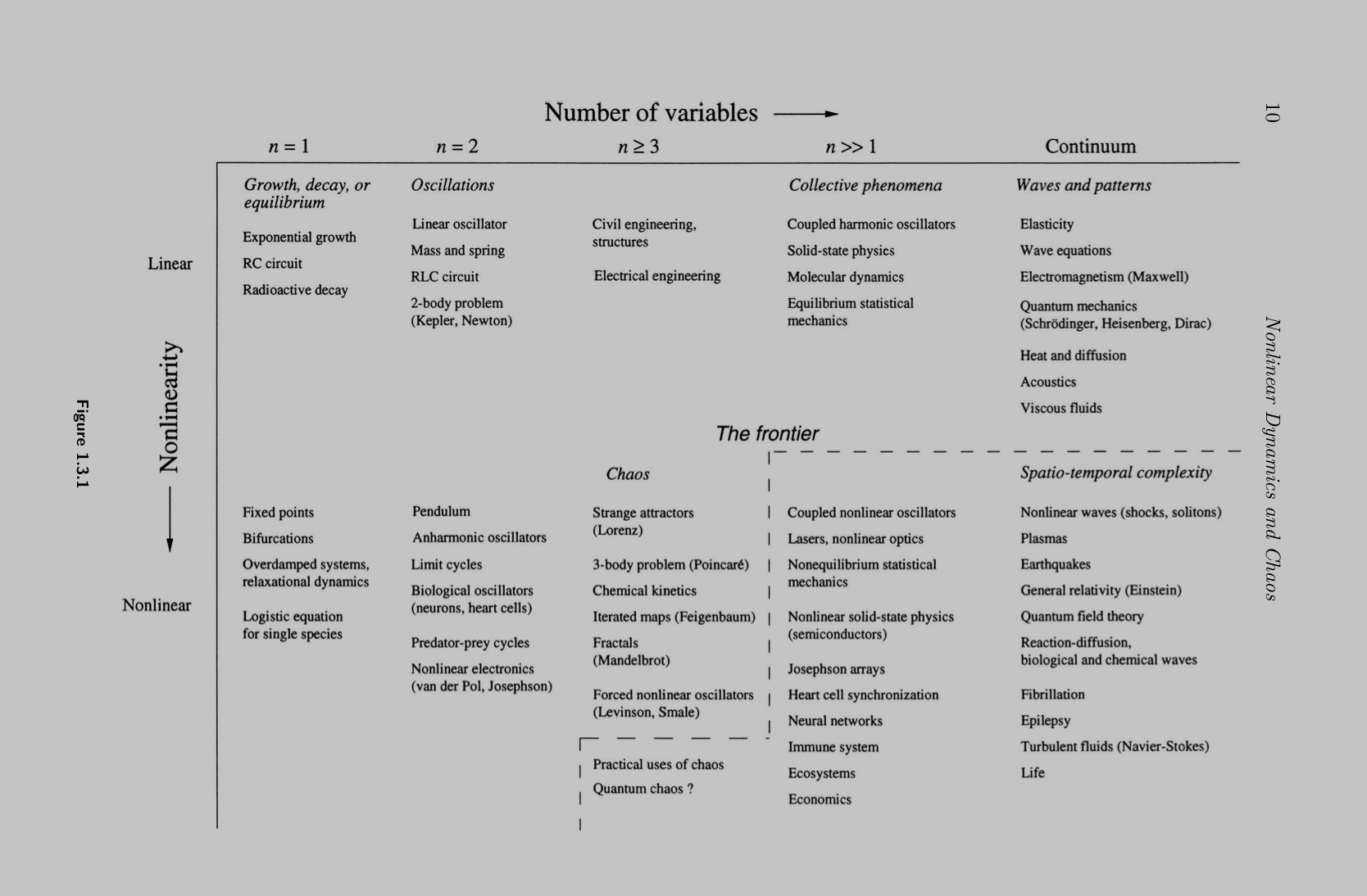
Figure: A matrix of models organized by number of variables (columns) and degree of nonlinearity (rows). Linear models with few variables (upper left) are the simplest; nonlinear models with many variables or continuous dimensions (lower right) represent the frontier of modeling complexity. Adapted from Strogatz (2015).

Description vs. Explanation

A descriptive model summarizes a pattern in data. It tells you the shape of a function and the values of its parameters. An explanatory (or mechanistic) model proposes a process that generates the pattern. Both are valuable, but they answer different questions.

Mazur's hyperbolic discounting function describes how subjective value declines with delay. A process model that specifies why hyperbolic decay occurs (e.g., via memory mechanisms or competing temporal representations) would explain it (e.g., Kileen's timing tied to reinforcement state and arousal; Shull's independent timer and bout-and-pause structure). Much of behavior science currently operates at the descriptive level. Pushing toward explanation is one of the frontiers where modeling can contribute.

Parameters vs. Variables

A variable is a quantity that changes across observations or conditions (e.g., delay to reinforcement, response rate). A parameter is a quantity that is fixed within a model but may differ across individuals or conditions (e.g., the sensitivity parameter in the generalized matching equation; the rate whereby delay or probability reduces the value of a reinforcer). Parameters are typically estimated from data.

Understanding the distinction is critical: when you fit a model, you are estimating parameters; when you use the model to predict, you are computing values of variables.

Curve Fitting vs. Mechanistic Modeling

Curve fitting finds the parameter values that make a given equation best describe a dataset. Curve fitting is a tool, not a theory. The fact that a hyperbola fits discounting data well does not, by itself, explain why discounting is hyperbolic.

Mechanistic modeling goes further by proposing processes whose operation produces the observed functional form. Both activities are legitimate parts of the modeling enterprise, but they should not be confused.

Model Families Overview

Over the coming weeks, we will encounter several families of models:

Algebraic models express relationships as equations involving arithmetic operations, powers, and standard functions. The matching law and discounting functions are algebraic models. They are solved by substitution and algebra.

Differential equation models express relationships in terms of rates of change. The Rescorla-Wagner model, in its continuous form, is a differential equation. These models describe how a system evolves over continuous time and are central to dynamical systems approaches.

Probabilistic models treat outcomes as random variables governed by probability distributions. Maximum likelihood estimation, Bayesian models, and many statistical frameworks fall here. They are useful whenever data contain noise, which is almost always.

Computational models specify algorithms rather than equations. Agent-based models, Monte Carlo simulations, and reinforcement-learning algorithms are computational. They excel at capturing emergent phenomena that arise from the iterative interaction of simple rules.

Machine learning models prioritize predictive accuracy, often at the expense of interpretability. Neural networks, random forests, and support vector machines are examples. They are powerful tools for pattern detection but can be difficult to interpret in behavioral terms without additional work (e.g., feature importance plots; ablation strategies).

Applying the 8-Step Framework

This section walks through each step of the 8-step modeling framework using a common example in behavior science: modeling the rate of lever pressing by a rat on a variable-interval (VI) schedule of food reinforcement.

Step 1: Get the behavioral phenomenon clearly in mind. A food-deprived rat is placed in an operant chamber equipped with a lever. Presses on the lever contact reinforcemen with food pellets according to a VI schedule. Over many sessions, the rat's response rate stabilizes. We want to model the relationship between the programmed reinforcement rate and the observed response rate.

Step 2: Define the behavioral processes and scope of the model. We will model steady-state response rate as a function of reinforcement rate. We will not model acquisition, extinction, or within-session changes. The model covers a single operant on a single schedule.

Step 3: Identify the behavioral principles and quantitative laws. Herrnstein's single-alternative matching law proposes that response rate is a hyperbolic function of reinforcement rate. This is our candidate law.

Step 4: State all simplifying assumptions. We assume the organism is at steady state. We assume a single source of measured reinforcement and a constant background level of extraneous reinforcement. We assume the critical establishing operation (i.e., food deprivation) is constant across conditions.

Step 5: Write the model verbally, then mathematically. Verbally: Current response rate equals the ratio of the obtained reinforcement rate to the sum of the obtained reinforcement rate and the extraneous reinforcement rate, with an upper bound response rate controlled by the max response rate physically possible. Mathematically:

$R = \frac{k \cdot r}{r + r_e}$

where $R$ is response rate, $r$ is reinforcement rate for the target response, $r_e$ is extraneous reinforcement rate, and $k$ is the asymptotic response rate.

In plain language: the equation says that as reinforcement rate increases, response rate increases toward a ceiling ( $k$ ), but with diminishing returns. The parameter $r_e$ controls how quickly responding approaches that ceiling.

Step 6: Verify dimensional consistency. $R$ is in responses per minute. $k$ is in responses per minute. $r$ is in reinforcers per minute. $r_e$ is in reinforcers per minute. The ratio $\frac{r}{r + r_e}$ is dimensionless (reinforcers per minute divided by reinforcers per minute). Therefore, the right side has units of responses per minute, matching the left side.

Step 7: Specify starting values and constraints. $k$ must be positive (you cannot have a negative response rate). $r_e$ must be positive. The model applies to VI schedule performance after responding has reached a stable state, typically after at least 20--30 sessions at each reinforcement rate.

Step 8: Check the math, test against data, and derive predictions. Verify: At $r = 0$ , $R = 0$ (no reinforcement yields no responding). As $r$ becomes very large, $R$ approaches $k$ (there is a ceiling on response rate). These are qualitatively sensible. Validate: Fit the equation to data from multiple VI schedule values and assess goodness of fit. Solve: Given estimated $k$ and $r_e$ , predict response rate at any new reinforcement rate.

Worked Example: $R = k \cdot t$

Consider the simplest possible behavioral model: cumulative responses as a linear function of time.

The Model

$R = k \cdot t$

where:

$R$ is the cumulative number of responses
$k$ is the response rate (responses per unit time), a constant
$t$ is elapsed time

In plain language: if you know how fast the organism is responding ( $k$ ), you can predict how many total responses will have occurred by any given time ( $t$ ) simply by multiplying. The model treats responding as a steady rate, kind of like water constantly streaming from a faucet filling a bucket.

Walking Through All 8 Steps

Step 1: Get the behavioral phenomenon clearly in mind. An organism is responding on some schedule. We observe that over a session, responses accumulate. We want to describe the cumulative record (i.e., the running total of responses as a function of time).

Step 2: Define the behavioral processes and scope. We model only the accumulation of responses over time within a single session. We do not model what maintains responding, how responding was acquired, or what happens between sessions.

Step 3: Identify behavioral principles and quantitative laws. We invoke the simplest possible assumption: the organism responds at a constant rate. This is the defining feature of steady-state VI schedule performance, at least as an approximation.

Step 4: State all simplifying assumptions. (a) Response rate is constant throughout the session. (b) There are no pauses, warm-up effects, or satiation effects. (c) Each response is identical and countable. (d) Time is measured continuously from session onset.

Step 5: Write the model verbally, then mathematically. Verbally: The cumulative number of responses equals the response rate multiplied by the elapsed time. Mathematically: $R = k \cdot t$ .

Step 6: Verify dimensional consistency. $R$ is in responses (count). $k$ is in responses per minute. $t$ is in minutes. Responses per minute multiplied by minutes equals responses. The units are consistent.

Step 7: Specify starting values and constraints. At $t = 0$ , $R = 0$ (no responses have occurred at the start of the session). $k$ must be non-negative. The model applies from session onset ( $t = 0$ ) to session end ( $t = T$ ), and only during periods when the constant-rate assumption is reasonable.

Step 8: Check the math, test against data, and derive predictions. Verify: The model predicts a straight-line cumulative record. If $k = 2$ responses/min and $t = 30$ min, then $R = 60$ responses. Validate: Compare the predicted straight line to actual cumulative records. In practice, real cumulative records show local variability (pauses, bursts), so the linear model will fit the overall trend but not the fine grain. Solve: Given an estimate of $k$ from observed data (e.g., total responses divided by total time), predict cumulative responses at any time point.

This is obviously a simplification. Real organisms pause, accelerate, and decelerate. But the linear model serves as a useful baseline. Deviations from linearity are informative: they point toward phenomena (satiation, ratio strain, schedule effects) that a more complex model would need to capture.

Assumptions and Limitations

The linear model $R = k \cdot t$ assumes:

Steady-state responding: The rate is constant. This is approximately true for well-trained organisms on VI schedules during the middle portion of a session, but it is rarely true at the start (warm-up) or end (satiation) of a session.
Linearity: Cumulative responses grow proportionally with time. Nonlinear growth (e.g., negatively accelerated curves during satiation) violates this assumption.
Single response class: The model counts one type of response. If the organism engages in competing behaviors, the model does not account for them.
No measurement error: Every response is detected and counted. In practice, recording equipment has limits.

Importantly, all of the above limitations should be considered the boundaries of the model as opposed to flaws. Every model is incomplete and has boundary conditions under which it no longer performs well. Practically building and using models involves knowing what the boundary conditions are, when they matter, and when you need to do something about it.

Connection to Empirical Behavior Science

The cumulative record is one of the oldest and most characteristic tools of the experimental analysis of behavior. Skinner used it to visualize response patterns under different schedules of reinforcement. The linear model $R = k \cdot t$ corresponds to the idealized cumulative record for a VI schedule: a straight line whose slope reflects response rate.

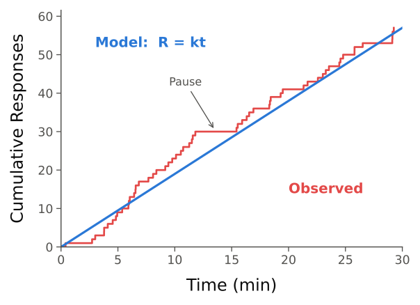
Idealized versus observed cumulative record

Figure: The linear model $R = k \cdot t$ (blue) predicts a straight-line cumulative record with slope $k$ . A real record (red) tracks the same overall slope but contains pauses and bursts the model deliberately omits. The model is wrong in the fine grain yet useful for the trend, and the deviations point to phenomena a richer model would need to capture.

More broadly, this week's introduction connects to the entire tradition of quantitative analysis in behavior science. The field has always valued prediction and control. Mathematical models make prediction explicit and testable. The 8-step framework provides a systematic method for constructing models that are clear, testable, and connected to behavioral principles.

Exercises for Reflection

Consider a behavioral phenomenon you study or find interesting. What would Step 1 (getting the phenomenon clearly in mind) look like for that phenomenon? What features would you need to observe and describe before attempting to model it?
The linear model $R = k \cdot t$ is almost certainly wrong for any real dataset if examined closely enough. In what sense can a model be both "wrong" and "useful"? What criteria would you use to decide whether a wrong model is still worth using?
What is the difference between fitting a curve to data and understanding the process that produced the data? Can you think of examples from behavior science where a good curve fit was mistaken for a good explanation?
The 8-step framework asks you to state your assumptions explicitly (Step 4). Why might this be the most important step? What are the consequences of unstated assumptions in a published model?

Key Readings

Critchfield and Reed (2009) examined what it means to "translate" from quantitative models of basic behavioral processes to applied contexts. The authors argue that translation is not simply applying a laboratory equation to a clinical setting. Rather, translating models is a principled process of identifying which features of a quantitative model carry over to new domains (i.e., its functional form, its parameters, its boundary conditions). This paper makes explicit that quantitative models are not just tools for curve fitting; they are vehicles to move knowledge from basic to applied science. Doing so requires understanding the model's structure as well as its output.

Dallery and Soto (2013) provided a comprehensive overview of how quantitative models describe environment-behavior relations across a range of basic behavioral phenomena. They distinguished between descriptive models that summarize data patterns and functional models that propose mechanisms, and they articulated the minimum requirements a quantitative model must meet: specify variables, parameters, and the functional form linking them. For this course, this chapter serves as a foundational reference that catalogs the major quantitative regularities in behavior analysis and demonstrates that the field already possesses a rich tradition of formal modeling, even if that tradition is not always recognized as such.

Cox (2026) argued that behavior is typically under multiple simultaneous sources of control (e.g., stimulus, motivational, historical) and that traditional analytic approaches often handle these sources one at a time rather than jointly. The paper introduced vector and matrix representations as tools for formalizing the multiple control of behavior within a single quantitative framework. This reading connects directly to the course's emphasis on mathematical formalization. Specifically, it shows that moving from verbal descriptions of "multiple control" to precise mathematical representations reveals structure that verbal accounts obscure, and it previews the kind of mathematical thinking that will be developed throughout the semester.

Reading Guide

Critchfield & Reed (2009)

Why has quantitative analysis become increasingly central in basic behavior analysis, according to the authors?
What do the authors mean by "translation" in the context of quantitative models, and how is this different from creating clinical applications?
What risk do the authors identify if basic and applied branches of behavior analysis stop "speaking the same language"?
What are the four core features of a quantitative model as outlined in the article?
How do fitted parameters contribute to the explanatory power of a quantitative model?
How does the use of equations in behavioral science provide greater precision than narrative descriptions alone?
What considerations must be made when choosing a quantitative model for translation?
What challenges arise when applying laboratory-based equations to field data?
Why might fitted parameters be more important than just verifying the presence of a core functional relation?
What examples do the authors give of everyday behaviors that can be modeled using quantitative principles like the matching law or delay discounting?
What constitutes a "standard equation," and how do they help guide translational work?
What does it mean for a model to offer "unique, testable predictions," and why is this a gold standard for theoretical utility?
How can translational work using quantitative models lead to improvements in both science and practice, even if the models are not perfect?

Dallery & Soto (2013)

What is the primary purpose of using quantitative models in behavior analysis according to Dallery & Soto?
How do the authors define a quantitative model?
Why do the authors argue that narrative and quantitative models are complementary?
What do the authors describe as the minimum requirements for a quantitative model?
What is the difference between descriptive and functional models?
Why is it important to include parameters in quantitative models?
What does a "good fit" indicate when using quantitative models?
Why do the authors caution against equating model fit with explanatory power?
What are some benefits of quantitative models in applied settings?
How can quantitative models contribute to individualized treatment planning?
How do the authors link model development to theory-building in behavior analysis?
Why is simplicity (parsimony) a valued feature in model selection?
How do quantitative models promote scientific communication?

Cox (2026)

What is meant by "multiple control" in behavior analysis?
Why does the author argue that a comprehensive understanding of behavior requires analyzing multiple control?
What is one limitation of traditional approaches to analyzing multiple control?
How do visual models like the "Four-Term Contingency" fall short?
According to the author, what is a model in the context of behavioral science?
Why are models necessary for advancing the science of behavior?
What are some general forms that models can take in behavior analysis?
What distinguishes a model from a theory or conceptual framework?
Why does the author emphasize the need for formalization in modeling multiple control?
How can mathematical models help resolve ambiguity in multiple control situations?
What is the potential benefit of adopting mathematical tools like matrices and vectors in behavioral analysis?
What does the author suggest is the next frontier for analyzing multiple control?

References

Cox, D. J. (2026). Of models, vectors, and matrices: Advancing analyses of the multiple control of behavior. Advances in the Experimental Analysis of Behavior. Pre-print: https://doi.org/10.13140/RG.2.2.11144.94723

Critchfield, T. S., & Reed, D. D. (2009). What are we doing when we translate from quantitative models? The Behavior Analyst, 32(2), 339--362. https://doi.org/10.1007/BF03392197

Dallery, J., & Soto, P. L. (2013). Quantitative description of environment-behavior relations. In G. J. Madden (Ed.), APA handbook of behavior analysis: Vol. 1. Methods and principles (pp. 219--249). American Psychological Association. https://doi.org/10.1037/13937-010

Gudmundsson, A. (2020). Volcanotectonics: Understanding the structure, deformation and dynamics of volcanoes. Cambridge University Press. https://doi.org/10.1017/9781139176217

Strogatz, S. H. (2015). Nonlinear dynamics and chaos: With applications to physics, biology, chemistry, and engineering (2nd ed.). Westview Press.

Key Takeaways

What is a model? A formal (mathematical or computational) representation of a system or process, built to predict, explain, or both.
Types of models: Verbal, mathematical, computational, and simulation. These overlap in practice.
Key distinctions: Description vs. explanation; parameters (estimated) vs. variables (observed or manipulated); curve fitting (tool) vs. mechanistic modeling (theory).
Model families for this course: Algebraic, differential equation, probabilistic, computational, and machine learning.
The 8-step framework: (1) Understand the phenomenon. (2) Define scope. (3) Identify principles and laws. (4) State assumptions. (5) Write the model in words, then symbols. (6) Check units. (7) Specify initial/boundary conditions. (8) Verify, validate, solve.
Worked example: $R = k \cdot t$ models cumulative responding as a linear function of time. The slope $k$ is the response rate. The model assumes constant-rate responding and serves as a baseline against which more complex models can be compared.
Takeaway: Modeling is a disciplined activity with a clear structure. The 8-step framework provides that structure and will be applied to every model encountered in this course.

Introduction to Modeling in Behavior Science