Week 10: Dynamical Systems Models

Why This Topic Matters

Behavior unfolds in real time. An organism does not "have" a response rate the way a rock has a mass. Rather, response rates emerge, shift, accelerate, and sometimes collapse across seconds, minutes, and sessions. Whenever we say that behavior is "acquired", "extinguished", or "in transition", we imply a dynamical process. That is, a process whose state changes over time in systematic and reliable way such that it can be described by scientists according to one or more rules. Dynamical systems theory provides the mathematical language for such processes.

Many behavioral phenomena also involve feedback loops. A response produces a reinforcer, which alters the probability of future responding, which changes the reinforcement rate, and so on. Stability, instability, oscillation, and abrupt transitions are useful vocabulary in dynamical systems theory. And, these terms map directly onto behavioral phenomena in steady-state behavior (stability), behavioral variability (instability), cyclic patterns in adjunctive behavior (oscillation), and the sudden shifts observed in resurgence or relapse (abrupt transitions). Formalizing these as dynamical models lets us make quantitative predictions about temporal trajectories as well as behavioral stability.

Core Concepts

State Variables

State variables are the quantities that define the system at any moment. In a behavioral model, examples of state variables might be momentary response rate (responses per minute), trajectory of response rate, cumulative reinforcers earned, the historical covariance of a stimulus–response association, and the physical value of any functionally relevant environmental stimulus (e.g., the hue of red behind a red key in an operant chamber). At any given instant, the values of all state variables together specify the complete "status" of the behavior-environment system.

Phase Space and Phase Portraits

The collection of all possible values of the state variables defines the phase space (or state space). For a single state variable like response rate, the phase space is a line of all values response rate can take. For two interacting variables, it is a plane of all combinations the two variables can take (e.g., the x-y plane commonly observed when graphing). A phase portrait is a graphical representation of trajectories through phase space, showing how the system evolves from various initial conditions. Arrows on the portrait indicate the direction and speed of change.

Equilibrium Points

An equilibrium point (or fixed point) is a state where the system, once there, remains there unless energy from outside the system moves it. That is, the rate of change in the system is zero. In behavioral terms, this corresponds to steady-state performance. There are several types of equilibria:

Stable equilibrium: the system returns to the point after a small perturbation. Examples include:
- A marble at the bottom of a bowl.
- A reversible chemical reaction at equilibrium, where forward and reverse rates are equal and concentrations hold constant.
- Body temperature returning to its set point after exercise.
- A population at its carrying capacity after a drought year.
Unstable equilibrium: any small perturbation drives the system away. Examples include:
- A marble balanced on a hilltop.
- A reacting mixture held exactly at its ignition temperature, where heat produced by the reaction equals heat lost to the surroundings. A slightly higher temperature runs away and a slightly lower one dies out.
- A neuron's membrane potential held exactly at firing threshold, where a slight depolarization triggers a spike and a slight hyperpolarization decays back to rest.
- A population sitting exactly at its minimum viable size, above which it grows and below which it declines to extinction.
Saddle point: stable in some directions but unstable in others (possible in systems with two or more state variables). Examples include:
- A marble on a mountain pass, which returns if pushed toward either peak but rolls away if pushed toward either valley.
- A chemical transition state, which is a minimum in every direction on the potential energy surface except the reaction coordinate, along which it is a maximum.
- The coexistence point of two strongly competing species, where a trajectory that starts with both species near that point ends with one species excluding the other. Which one survives depends on which side of the point the system started on.

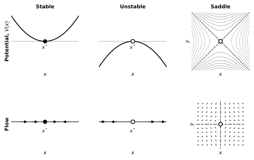
The three kinds of equilibrium drawn as potentials

Figure: The three kinds of equilibrium drawn as potentials with their flows beneath.

Attractors and Limit Cycles

Attractors are states or sets of states toward which the system tends over time. A stable equilibrium is the simplest attractor. But dynamical systems can also exhibit sustained oscillations that the system settles into regardless of initial conditions (i.e., limit cycles). In behavioral terms, a limit cycle might describe a response pattern that waxes and wanes rhythmically within or across sessions.

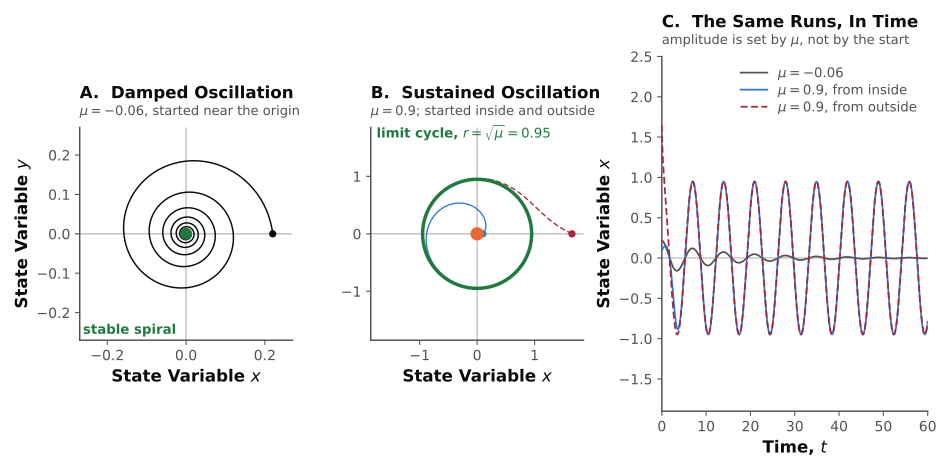
A damped oscillation and a limit cycle

Figure: An oscillation whose amplitude decays to zero and one whose amplitude does not, from the same family of equations. In polar coordinates the system is $dr/dt = r(\mu - r^2)$ and $d\theta/dt = \omega$ , with the plotted state variables $x = r\cos\theta$ and $y = r\sin\theta$ and $\omega = 0.9$ throughout.

Bifurcations

Bifurcations are qualitative changes in the system's behavior that occur when a parameter crosses a critical value. For example, a stable equilibrium might suddenly become unstable when a reinforcement rate drops below a threshold, causing a significant shift in behavioral allocation. Bifurcation analysis helps identify the parameter values where such transitions occur.

The simplest behavioral case is the logistic model with a constant rate of disruption $h$ removed at every moment:

\frac{dx}{dt} = r \cdot x \cdot \left(1 - \frac{x}{K}\right) - h

For small $h$ this has two equilibria. The upper one is stable and is the steady-state rate that the organism maintains under that level of disruption. The lower one is unstable and is a threshold: responding that starts below it decays to zero. As $h$ increases the two move toward each other, and at $h_c = rK/4$ they meet and disappear. Beyond that value $dx/dt$ is negative at every rate, so responding declines to zero no matter where it starts. The steady state does not shrink continuously to zero; it exists up to $h_c$ and then ceases to exist. Two equilibria colliding and annihilating in this way is a saddle-node bifurcation, and it is the same structure as the harvesting model in Orloff (2024).

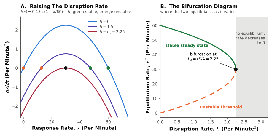
Saddle-node bifurcation in the logistic model under disruption

Figure: Adding a constant disruption rate $h$ to the worked example ( $r = 0.15$ , $K = 60$ ) up to the value at which the steady state ceases to exist. Left: the rate of change against response rate for several values of $h$ , with the two equilibria where each curve crosses zero. Right: the equilibria plotted against $h$ , meeting at $h_c = rK/4$ .

Some Terms Before the Math

The next section uses five terms that may be new to you. Feel free to skip through this if these terms are familiar.

Partial derivative: A derivative is a slope and describes how fast one quantity changes per unit change in another. With two state variables (e.g., response rate $x$ and obtained reinforcement rate $y$ ), the rate of change of $x$ depends on both. A partial derivative quantifies the slope of one variable at a time while holding the other fixed. $\partial f / \partial y$ is how much the rate of change of $x$ shifts when $y$ increases by one unit and $x$ does not move. The notation is the only new part; the operation is the derivative used in Weeks 3 and 8.

Jacobian matrix: A matrix is a table of numbers arranged in rows and columns. The Jacobian matrix is the table of all the partial derivatives, one row per state variable and one column per variable that state variable can interact with. For two variables it has four entries:

How $x$ affects its own rate of change,
How $y$ affects the rate of change of $x$ ,
How $x$ affects the rate of change of $y$ , and
How $y$ affects its own.

Evaluated at an equilibrium, each entry is a number. So the Jacobian is a record of every local feedback in the system at that point in the phase space. The diagonal entries are self-feedback and the off-diagonal entries are cross-feedback.

Eigenvector and eigenvalue: A perturbation from an equilibrium has a direction (which variables were pushed, and by how much relative to one another) and a size. In general the Jacobian both stretches a displacement and rotates it. For most matrices there are a few directions along which a displacement is stretched or shrunk without being turned. These are called the eigenvectors. The rate of that stretching or shrinking is the eigenvector's eigenvalue. A two-variable system has two eigenvectors and two eigenvalues. Any displacement can be split into a part along each eigenvector, each part grows or decays at its own eigenvalue's rate, and the two parts do not interact. That is why stability can be understood from the eigenvalues alone. A negative eigenvalue marks a direction along which perturbations decay, a positive one marks a direction along which they grow.

Real and imaginary parts: The formula for the eigenvalues contains a square root, and when the quantity under it is negative the eigenvalues are complex numbers, written as a real part plus an imaginary part. The two parts have separate jobs. The real part is the growth or decay rate, exactly as above. The imaginary part is a rotation rate. That is, the displacement circles the equilibrium while it grows or shrinks, which produces a spiral in a phase portrait and an oscillation in a time series. Stability depends only on the real part.

Trace and determinant: For a two-by-two matrix these are two ways we can summarize the entire table. The trace is the sum of the diagonal entries, the total amount of self-feedback. The determinant is the product of the diagonal entries minus the product of the off-diagonal entries, the dominance of self vs. interactive feedback. Both eigenvalues can be computed from the trace and the determinant (see below).

Linear Stability Analysis

Linear stability analysis determines the stability of an equilibrium by examining the eigenvalues of the Jacobian matrix evaluated at that point. It works because close to an equilibrium the nonlinear system is well approximated by a linear one, and linear systems can be solved exactly.

Let's start with a system that has one variable. We can write the state of this system as a displacement from the equilibrium:

u = x - x^*

where $x$ is the rate of change at equilibrium and $x^*$ is the rate of change of our system at point $u$ . To understand the dynamics, we can expand $f$ about $x^*$ . Because $f(x)=0$ by the definition of the system being at equilibrium, the leading term vanishes and we get:

\frac{du}{dt} = f'(x^*) \cdot u + O(u^2)

If we make our displacement really tiny, the $u^2$ term becomes even smaller and, thus, negligible. The solution then becomes:

u(t) = u(0)e^{f'(x^*)t}

The sign rule tells us that displacement shrinks when $f'(x^*) < 0$ and grows when $f'(x^*) > 0$ . The magnitude of $f'(x^*)$ sets the time scale. Specifically, the displacement changes by a factor of $e$ every $1/|f'(x^*)|$ units of time, so a more negative derivative means a faster return.

With two or more state variables the single derivative becomes a matrix of partial derivatives. For the system $\frac{dx}{dt} = f(x, y)$ and $\frac{dy}{dt} = g(x, y)$ , the Jacobian evaluated at the equilibrium $(x^*, y^*)$ is

J = \begin{pmatrix} \partial f / \partial x & \partial f / \partial y \\ \partial g / \partial x & \partial g / \partial y \end{pmatrix}

Each entry is a sensitivity. The diagonal entries give each variable's effect on itself and the off-diagonal entries give the effect of each variable on the other. If both off-diagonal entries are zero the variables do not interact and each can be analyzed separately.

An eigenvector of $J$ is a direction in which the linearized flow does not rotate, and its eigenvalue ( $\lambda$ ) is the rate at which a displacement along that direction grows or shrinks, as $e^{\lambda t}$ . A two-variable system has two eigenvalues, so a displacement splits into two components that each grow or decay at their own rate (one in the $x$ direction and one in the $y$ direction). Stability, therefore, depends on all the eigenvalues at once:

If all eigenvalues have negative real parts, every component decays and the equilibrium is stable.
If any eigenvalue has a positive real part, the component along that eigenvector grows and the equilibrium is unstable regardless of the other components.
Complex eigenvalues come in conjugate pairs, and the imaginary part is a rotation rate. The real part still determines stability, so the trajectory approaches or departs from the equilibrium along a spiral rather than a straight path.
If the largest real part is exactly zero, the linearization cannot determine whether the point is stable or unstable, and the nonlinear terms it discarded decide. This is why the three types above are exhaustive only when no eigenvalue has a real part of zero.

An equilibrium with one positive and one negative eigenvalue is the saddle described above. Displacements along one eigenvector decay while displacements along the other grow.

For a $2 \times 2$ Jacobian, we can calculate the eigenvalues from the trace and the determinant. The trace ( $\tau$ ) is the sum of the diagonals. That is, the value in the first row and first colum ( $J_{11}$ ) and the value in the second row and second column ( $J_{22}$ ). As an equation: $\tau = J_{11} + J_{22}$ .

The determinant ( $\Delta$ ) calculates the interaction between the self-feedback ( $J_{11}J_{22}$ ) and the interaction among the variables ( $J_{12}J_{21}$ ). As an equation: $\Delta = J_{11}J_{22} - J_{12}J_{21}$ .

The eigenvalues ( $\lambda$ ) can then be calculated using the following equation:

\lambda = \frac{\tau \pm \sqrt{\tau^2 - 4\Delta}}{2}

A negative determinant ( $\Delta$ ) gives one positive and one negative eigenvalue, which is a saddle. A positive determinant ( $\Delta$ ) with a negative trace ( $\tau$ ) is stable. A positive determinant ( $\Delta$ ) with a positive trace ( $\tau$ ) is unstable.

When $\tau^2 < 4\Delta$ the square root is imaginary and the equilibrium is a spiral. The cases the linearization cannot settle sit on the axes of this classification:

$\tau = 0$ with $\Delta > 0$ gives a purely imaginary pair, so trajectories circle the equilibrium rather than approaching or leaving it
$\Delta = 0$ gives a zero eigenvalue

Main Model Families

ODEs vs. Difference Equations

Dynamical models can be described by ordinary differential equations (ODEs) for continuous-time processes or as difference equations for discrete-time (trial-by-trial; session0by-session) processes. ODEs use derivatives ( $\frac{dx}{dt}$ ) to describe instantaneous rates of change, while difference equations use update rules ( $x_{n+1} = f(x_n)$ ) to describe change from one discrete step to the next. Both formulations describe how the state at the next moment depends on the current state.

Single ODE Models

The simplest dynamical model tracks a single state variable over continuous time:

\frac{dx}{dt} = f(x)

This says that the rate of change of $x$ at any instant is some function of the current value of $x$ .

A classic example is the logistic growth equation as a model of response acquisition:

\frac{dx}{dt} = r \cdot x \cdot \left(1 - \frac{x}{K}\right)

Here $x$ is response rate, $K$ is the asymptotic rate (maximum possible response rate), and $r$ is the rate at which responding is acquired. When responding is low relative to the maximum possible, the response rate accelerates approximately exponentially in this model. As $x$ approaches $K$ , the factor $(1 - x/K)$ shrinks toward zero, decelerating growth. The result is the classic S-shaped (sigmoidal) acquisition curve.

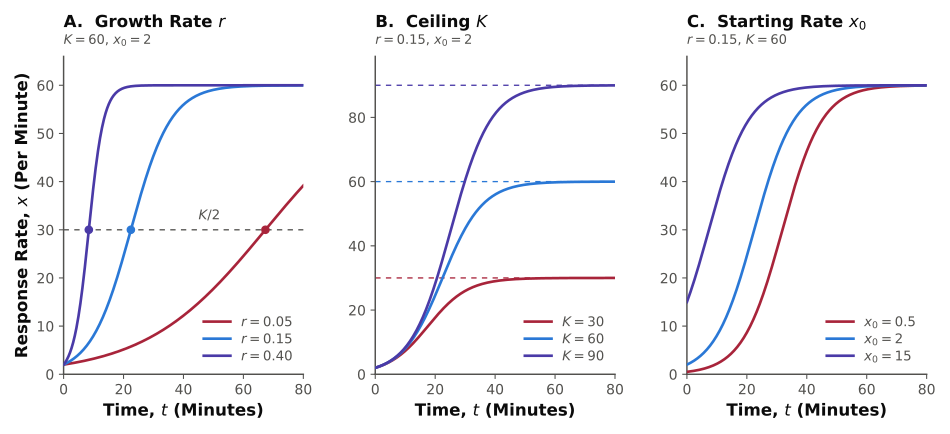
Logistic acquisition curves across values of r, K, and the starting rate

Figure: The logistic trajectory as $r$ , $K$ , and the starting rate are varied one at a time.

Coupled ODE Systems

When two or more behavioral processes interact, we need coupled equations (i.e., equations that interact with one another). A Lotka–Volterra analog for two competing responses takes the form:

\frac{dx}{dt} = r_x \cdot x \cdot \left(1 - \frac{x + a \cdot y}{K_x}\right)

\frac{dy}{dt} = r_y \cdot y \cdot \left(1 - \frac{y + b \cdot x}{K_y}\right)

Here $x$ and $y$ are the rates of two competing responses. The parameters $r_x$ and $r_y$ are growth rates set by the reinforcement each response contacts, and $K_x$ and $K_y$ are the rates each response would reach if the other were absent. The terms $a$ and $b$ measure cross-suppression: $a$ is the number of units of $x$ that one unit of $y$ displaces, and $b$ is the reverse. These capture mutual suppression where time and effort spent on one response reduce the other.

The self-limiting term in each equation is what makes a stable allocation possible. Written without it, as $dx/dt = a \cdot x - b \cdot x \cdot y$ and $dy/dt = c \cdot y - d \cdot x \cdot y$ , the interior equilibrium sits at $x^* = c/d$ and $y^* = a/b$ , where the Jacobian has zero trace and determinant $-ac$ . A negative determinant is a saddle, so responding never settles there and the model cannot describe a maintained allocation. Only the self-limiting form above has a stable interior equilibrium, and it sits where $x + a \cdot y = K_x$ and $b \cdot x + y = K_y$ .

That equilibrium exists and is stable when $a \cdot b < 1$ , which is to say when each response suppresses the other less than it suppresses itself. This structure can model concurrent-schedule performance where responding on two operanda competes for behavioral allocation, and the dynamics of behavioral momentum theory where response rate and reinforcement context interact.

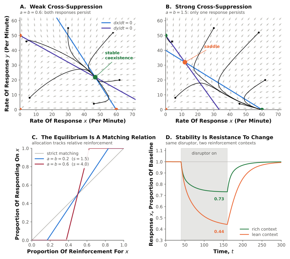
Phase plane for two competing responses, with matching and resistance to change

Figure: The competition model read four ways. (A) With weak cross-suppression ( $a = b = 0.6$ ) the interior equilibrium is stable and both responses persist. (B) With strong cross-suppression ( $a = b = 1.5$ ) the same point is a saddle, so one response displaces the other, and which one wins depends on the starting rates. (C) Varying the reinforcement allotted to $x$ moves the stable equilibrium along a matching relation. Allocation tracks relative reinforcement, and the sensitivity is $s = (1 + a)/(1 - a)$ , set by the cross-suppression; the diagonal is strict matching. Outside the range in which both responses persist the model predicts exclusive choice. (D) A constant disruptor applied to $x$ for 120 time units in a rich context ( $r_x = 0.26$ ) and a lean one ( $r_x = 0.12$ ). The richer context falls to a higher proportion of its own baseline and returns to it faster, which is resistance to change.

Panels C and D recover two results from earlier weeks as properties of the same equilibrium. The location of the equilibrium is the matching relation of Week 2, obtained here as the allocation the system settles into rather than as a description fitted to steady-state data. The stability of that equilibrium is resistance to change: the eigenvalue governs how far a disruptor moves responding and how quickly it returns, which is the distinction Nevin and Grace (2000) draw between response rate and resistance to change. One caveat is worth stating. Because $a$ and $b$ are positive, the sensitivity $(1 + a)/(1 - a)$ is always at least 1, so competition of this form produces strict matching or overmatching. The undermatching usually obtained in concurrent schedules requires something this model omits, such as imperfect discrimination between the alternatives or a cost of switching.

Discrete Dynamical Systems

For trial-by-trial processes, we use difference equations:

x_{n+1} = f(x_n)

This says that the state on the next trial is some function of the state on the current trial. For instance, a learning rule might update associative strength after each trial based on prediction error (e.g., Rescorla-Wagner model). One way to describe difference equations is that they map the value of the current state of the system to the next state of the system (aka discrete maps). Discrete maps can exhibit rich dynamics including fixed points, periodic orbits, and even chaos, depending on the form of $f$ .

Rescorla-Wagner as a discrete map, with a cobweb construction

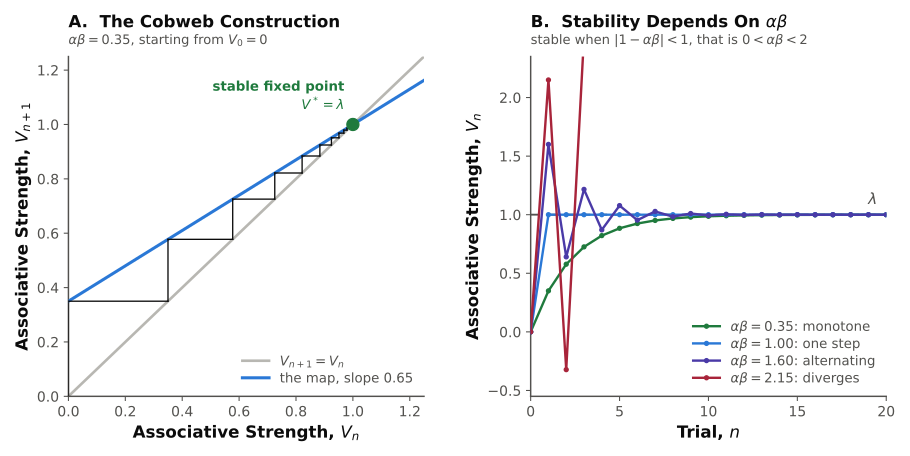
Figure: The Rescorla-Wagner update rule as a map and the influence of learning rate on stability.

Applying the 8-Step Framework

We next will walk through all eight steps for a dynamical model of operant response acquisition using the logistic ODE.

Step 1: Identify All Environmental and Behavioral Components of the Phenomenon

An organism is placed in an operant chamber with a lever. Initially, the rat rarely presses the lever. Over the course of a session, lever pressing increases. It increases first slowly, then rapidly, then gradually leveling off at a steady rate. We want a mathematical model that describes how response rate changes over time during this acquisition process.

Step 2: Define the Behavioral Principles, Processes, and Intended Scope of the Model

The process of interest is the change in response rate over time within a single extended session (or across sessions, with time measured cumulatively). The boundaries of the model include: one organism, one operandum (lever), one reinforcement schedule (e.g., continuous reinforcement), and no competing alternatives. We are not modeling the reinforcement mechanism itself, only the resulting trajectory of response rate.

Step 3: Write Down the Behavioral Principles, Known Quantitative Laws, and Functional Relationships

We adopt the logistic growth equation as the descriptive and predictive equation:

\frac{dx}{dt} = r \cdot x \cdot \left(1 - \frac{x}{K}\right)

This equation has two assumptions. First, that low-rate responding tends to accelerate (positive feedback from reinforcement). Second, that there is a ceiling rate $K$ imposed by physical constraints and schedule saturation. The dynamical change from low to high responding is driven by the term $r \cdot x$ , and is limitd by the factor $(1 - x/K)$ .

Step 4: State All Simplifying Assumptions Explicitly

Time is treated as continuous, even though responses are discrete events.
The environment is stationary (i.e., reinforcement schedule does not change, no disruptions).
Only a single operant response is modeled; no competing responses are considered.
The model is deterministic; stochastic variability in responding is ignored.
Parameters $r$ and $K$ are constants (they do not change with time or experience).
Motivational state is constant (i.e., no satiation or deprivation changes within the session).

Step 5: Write the Model Verbally, Then Express It Mathematically

In words: the rate of change of responding equals the current response rate multiplied by a change rate, reduced by a factor that approaches zero as the response rate approaches its maximum.

Mathematically:

\frac{dx}{dt} = r \cdot x \cdot \left(1 - \frac{x}{K}\right).

This is the balance equation, expressing the "input" to behavior change (reinforcement-driven increase, $r \cdot x$ ) against the "constraint" (maximum rate of responding, $1 - x/K$ ).

Step 6: Verify Dimensional Consistency

Let $x$ be in responses per minute (resp/min). Then $dx/dt$ is in resp/min $^2$ . $K$ is in resp/min, so $x/K$ is dimensionless, and $(1 - x/K)$ is dimensionless. Therefore $r$ must have units of min $^{-1}$ so that $r \cdot x \cdot (1 - x/K)$ yields resp/min $^2$ . Units check.

Step 7: Specify Starting Values and Constraints

The initial condition is $x(0) = x_0$ , where $x_0$ is the response rate at the beginning of the observation period. We also have the implicit boundaries that $x \geq 0$ (negative response rates are not meaningful) and $x \leq K$ (the ceiling).

Step 8: Check the Math, Test Against Data, and Derive Predictions

The logistic ODE has an exact analytical solution:

x(t) = \frac{K}{1 + \left(\frac{K - x_0}{x_0}\right) e^{-r t}}

This closed-form expression gives the response rate at any time $t$ given the parameters and initial condition.

Verification:

At $t = 0$ , $x(0) = K / (1 + (K - x_0)/x_0) = K / (K/x_0) = x_0$ . Correct.
As $t \to \infty$ , the exponential vanishes, giving $x = K$ . Correct. Taking the derivative and substituting back confirms the ODE is satisfied.

Validation would involve fitting this function to empirical acquisition data and assessing goodness of fit.

Worked Example

We model acquisition of lever pressing in a rat with the following parameter values:

$K = 60$ responses per minute (asymptotic rate)
$r = 0.15$ per minute (response-rate-increase parameter)
$x_0 = 2$ responses per minute (initial rate from occasional exploratory presses)

The analytical solution becomes:

x(t) = \frac{60}{1 + \frac{58}{2} \cdot e^{-0.15t}} = \frac{60}{1 + 29 \cdot e^{-0.15t}}

Equilibrium Analysis

To determine the equilibrium (i.e., steady state) response rate, the rate of change would be zero. That is, $dx/dt = 0$ . That would mean that $r \cdot x \cdot (1 - x/K) = 0$ . In turn, that yields two equilibria: $x = 0$ and $x = K = 60$ .

To assess stability, we compute $f'(x) = r(1 - 2x/K)$ :

At $x = 0$ : $f'(0) = 0.15 > 0$ (positive), so $x = 0$ is unstable. Any small amount of responding will increase.
At $x = 60$ : $f'(60) = 0.15(1 - 2) = -0.15 < 0$ (negative), so $x = 60$ is stable. The system returns here after perturbation.

Phase Portrait Description

On a horizontal axis labeled $x$ (response rate, 0 to 70), the function $f(x) = 0.15 \cdot x \cdot (1 - x/60)$ forms an inverted parabola passing through $x = 0$ and $x = 60$ and with a maximum at $x = 30$ .

For $0 < x < 60$ , $f(x) > 0$ , so $x$ increases (arrows point right on the number line). For $x > 60$ , $f(x) < 0$ , so $x$ decreases (arrows point left).

This confirms that $x = 0$ is unstable (arrows diverge) and $x = 60$ is stable (arrows converge).

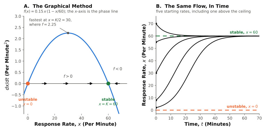
Flow on the line for the logistic model

Figure: The phase portrait described above.

Computing $x(t)$ at Specific Times

At $t = 10$ minutes:

x(10) = \frac{60}{1 + 29 \cdot e^{-1.5}} = \frac{60}{1 + 29 \times 0.2231} = \frac{60}{1 + 6.470} = \frac{60}{7.470} \approx 8.03 \text{ resp/min}

At $t = 20$ minutes:

x(20) = \frac{60}{1 + 29 \cdot e^{-3.0}} = \frac{60}{1 + 29 \times 0.0498} = \frac{60}{1 + 1.443} = \frac{60}{2.443} \approx 24.56 \text{ resp/min}

At $t = 30$ minutes:

x(30) = \frac{60}{1 + 29 \cdot e^{-4.5}} = \frac{60}{1 + 29 \times 0.0111} = \frac{60}{1 + 0.322} = \frac{60}{1.322} \approx 45.39 \text{ resp/min}

Trajectory Summary

The trajectory shows the classic sigmoidal shape. That is, slow initial growth (2 to about 8 resp/min in the first 10 minutes), rapid acceleration through the middle range (8 to 45 resp/min between minutes 10 and 30), and deceleration as the ceiling is approached. By about 45 minutes, the rate is within a few responses per minute of the asymptote at 60.

Connecting Backward: Static Models as Dynamical Snapshots

Many of the models from earlier weeks in this course describe equilibrium states. That is, the endpoints that a dynamical process settles into. Dynamical systems theory highlights that these static descriptions are snapshots of behavioral processes that dynamically change over time.

For example, the generalized matching equation (Week 2) describes the equilibrium allocation of behavior across concurrent schedules. From a dynamical perspective, matching is the stable attractor of a system where response allocation adjusts over time in response to relative reinforcement rates. The generalized matching law tells us where the system ends up. A dynamical model tells us how it gets there and how quickly it recovers from perturbation.

As another example, delay discounting (Week 2) can be viewed as a dynamic process of value change over time. As the delay to a reinforcer decreases (the moment of choice approaches), the subjective value of the delayed option increases along the discount function. This temporal unfolding of value is inherently dynamical and can produce preference reversals when two discount curves associated with the two choice options cross.

As a third example, demand curves (Week 3) describe equilibrium consumption at each price point. The exponential demand model tells us how much behavior is allocated at steady state for a given unit price. But, the demand equation does not describe the transient adjustments an organism makes when price changes. A dynamical model of demand would describe the trajectory from old equilibrium to new.

The Rescorla–Wagner model (Week 4) is also a discrete dynamical system. The update rule $\Delta V = \alpha \beta (\lambda - V)$ is a first-order difference equation. The associative strength $V$ is the state variable, and the prediction error $(\lambda - V)$ drives the system toward the equilibrium $V = \lambda$ . Everything we learn this week about stability and convergence applies directly to that learning rule.

Connecting Forward: Dynamics in Computation and ML

The dynamical systems perspective also extends to the computational and data-driven approaches covered in coming weeks.

Computational models (Week 11) implement dynamical rules as step-by-step algorithms. A simulation of the logistic acquisition model, for example, uses Euler's method or a Runge–Kutta solver to numerically integrate the ODE. Every computational model that updates state variables on each time step is, at its core, implementing a dynamical system.

Q-learning is a dynamical system that updates a table of action values. The Q-value update rule is:

Q(s,a) \leftarrow Q(s,a) + \alpha [r + \gamma \max_{a'} Q(s',a') - Q(s,a)]

This is a difference equation in which Q-values are state variables converging (under appropriate conditions) toward a fixed-point equilibrium. The learning rate $\alpha$ controls the speed of convergence, just as $r$ does in our logistic model.

Neural network training is gradient descent on a loss landscape which is a high-dimensional dynamical system. The weights are state variables, the loss function defines the landscape, and the learning rate governs step size. Concepts like attractors (local minima), saddle points, and bifurcations (sharp transitions in learned representations) carry over directly from what we covered this week.

Machine learning models (Week 12) can learn dynamical relationships from data. Recurrent neural networks and state-space models are explicitly designed to capture temporal dependencies. When we fit such models to behavioral time series, we are using data-driven methods to discover the dynamical rules governing behavior. This allows us to close the loop between theory-driven and data-driven modeling.

Plain-Language Interpretation

What the Logistic Equation Says in Words

The logistic equation, $\frac{dx}{dt} = r \cdot x \cdot (1 - x/K)$ , says that the rate at which responding speeds up depends on two things. First, how much responding is already happening (the $x$ term). This is a positive feedback loop as more responding generates more reinforcement, which generates more responding. Second, how much room is left to grow which is the term: $1 - x/K$ . As the organism approaches its maximum rate, further acceleration becomes harder. Perhaps the schedule delivers reinforcers less efficiently at high rates, or physical fatigue imposes limits, or the session has finite reinforcers available.

What Equilibrium Means Behaviorally

An equilibrium is a response rate at which there is no tendency to change. The stable equilibrium of the logistic equation at $x = K$ is the steady-state rate. If the organism is momentarily perturbed, the system will drift back to $K$ . Here perturbation might be a brief distraction that reduces response rate, or a burst of responding that temprarily (and unsustainably) increases it. This is the dynamical-systems formalization of what behavior analysts call "steady state".

Equilibrium is a property of the chosen state variables. At steady state the rate is constant while individual responses and reinforcers continue to occur, in the same way that a chemical reaction at equilibrium has constant concentrations while molecules continue to convert in both directions at equal rates. Chemists call this a dynamic equilibrium to distinguish it from a system in which nothing is happening. Whether a system counts as being at equilibrium depends on which variables were declared to be the state in Step 2 of the framework. As behavior analysts, we recognize that many different public and private stimuli can influence behavior (i.e., the multiple control of behavior). We can technically include as many variables as we want to, roll those values into the state of the current behavior-environment system, and use the techniques described above to solve for the dynamics and equilibrium of the system as we have defined it. The trick always comes back to validation. That is, it is easy to claim multiple control and the quantitative equations we assume to describe and predict that system. It is another thing altogether to collect the data, run the experiment, and validate the mathematical system we have created is correct.

What Stability Means

Stability means that the system returns to its equilibrium after a perturbation. A stable equilibrium acts like a valley. If you push the system away, it rolls back. In behavioral terms, a stable steady state is one that is robust to minor disruptions. The rat may pause briefly to groom, but lever pressing returns to its characteristic rate. The eigenvalue (or derivative) being negative at the equilibrium is the mathematical signature of this return.

What Instability of $x = 0$ Means

The instability of $x = 0$ means that even a tiny amount of responding ( $x_0 > 0$ ) will grow rather than collapse back to zero. Behaviorally, this captures the observation that acquisition tends to proceed once even a few responses contact reinforcement (note that this does not solve the problem of first instance). Zero responding is a precarious state as any perturbation away from it (an accidental lever press, a shaped approximation) initiates the acquisition process.

Assumptions and Limitations

The logistic model is a useful starting point, but it has important assumptions:

Continuous approximation: Real acquisition consists of discrete responses at variable intervals. The continuous ODE is an approximation that works best when response rates are moderate to high.
No competing behaviors: The model tracks a single response. In reality, organisms always have many alternative behaviors they can emit at any one point in time.
No satiation: Motivational state is assumed constant. In practice, within-session satiation can produce systematic decreases in responding.
Fixed ceiling: The asymptote $K$ is assumed constant, but in practice it may shift with extended training or changes in schedule parameters.
Deterministic: The model omits the substantial trial-to-trial variability evident in individual-organism data.
Phenomenological: The logistic equation describes the shape of acquisition without deriving it from reinforcement principles. A more mechanistic model might derive the growth rate from the specific schedule contingency, reinforcer magnitude, and an organism specific learning rule. The logistic equation is best understood as a descriptive first step.

Dynamical systems theory provides the tools for richer, more mechanistic models, but every additional complexity must be justified by what it adds in explanatory or predictive power.

Connection to Empirical Behavior Science

Dynamical systems models have been applied to several domains in behavior science:

Acquisition curves: Across many species and schedule types, acquisition curves often show sigmoidal shapes consistent with logistic or similar growth models. The logistic provides a two-parameter ( $r$ , $K$ ) summary of the acquisition trajectory. The single alternative matching equation extends this idea to account for additional sources of reinforcement.
Behavioral momentum theory: This framework has been formalized using coupled differential equations relating response rate to reinforcement context. Disruption is modeled as a perturbation, and resistance to change is linked to stability properties of the equilibrium. Higher reinforcement rates in a context produce a "deeper" attractor basin, meaning greater resistance to disruption.
Resurgence and relapse: These phenomena involve transitions between behavioral states that can be modeled as movements through phase space. When a previously reinforced response is placed on extinction while an alternative is reinforced, and then the alternative is also extinguished, the return to the original response can be described as the system moving toward a new attractor after a bifurcation in the reinforcement landscape.
Choice dynamics: Dynamical models of concurrent-schedule performance describe how response allocation evolves over time toward a stable matching equilibrium. The Lotka–Volterra-style competition model captures mutual suppression between alternatives, and the equilibrium of such a system can correspond to matching or undermatching depending on parameter values.

Exercises for Reflection

The logistic model treats responding as continuous, but actual responses are discrete events separated by inter-response times. Under what conditions is the continuous approximation reasonable, and when might a discrete-time model be preferable? What features of the data would help you decide?
The phase-portrait analysis showed that $x = 0$ is an unstable equilibrium. But in practice, many organisms placed in a new operant chamber with no shaping never begin pressing the lever. How might you modify the model to accommodate a "threshold" below which behavior does not spontaneously grow?
Behavioral momentum theory proposes that resistance to disruption is a function of the reinforcement context. How would you formalize "disruption" in a dynamical systems model? Would it be a change in a parameter, a perturbation to a state variable, or something else?
Consider a behavior that oscillates rather than reaching a stable steady state (e.g., adjunctive polydipsia that waxes and wanes within a session). What kind of dynamical structure (attractor type) might produce such oscillations, and what would the phase portrait look like?

Key Readings

Required:

Orloff (2024) introduces the mathematics of one-variable autonomous differential equations, which is the technical foundation for everything else this week. The notes define the phase line, show how to locate equilibria by solving $f(x) = 0$ , and develop the graphical method of reading stability off a plot of $f(x)$ against $x$ (i.e., where $f$ is positive the state moves right, where it is negative it moves left). The direction of the arrows on either side of an equilibrium determines whether it is stable or unstable. The logistic equation appears twice, first as a worked phase-line example and again in an appendix that derives the closed-form solution used in this week's worked example above. The final sections build bifurcation diagrams from a logistic-with-harvesting model, which is the same structure this chapter uses to model disruption. These notes are open courseware, licensed CC BY-NC-SA 4.0, and are posted with the week's readings.

Marr (1992) argues that behavior analysis has concentrated on steady-state description at the cost of the transitions between states, and that dynamical systems theory supplies the vocabulary the field needs to talk about those transitions. He works through state spaces, trajectories, attractors, and the possibility that some behavioral phenomena involve chaotic variation, rather than "noisy" or "stochastic" variation. He does this using a mechanical analog for molar behavior under changing reinforcement conditions and a treatment of concurrent schedules. The paper is written by a behavior analyst for a behavior-analytic audience, so it connects the mathematics in Orloff to the behavioral models in this chapter.

Nevin and Grace (2000) formalize behavioral momentum theory and separate two things that are easy to conflate: response rate, controlled by the response-reinforcer contingency, and resistance to change, controlled by the stimulus-reinforcer relation. In the vocabulary of this week the first is the location of an equilibrium and the second is its stability, which makes the paper a behavioral application of the stability analysis developed in Orloff. Read the target article, pages 73 to 90, not the commentaries.

Supplemental: Myerson and Miezin (1980) presented a kinetic model of choice that applies systems analysis to concurrent schedule performance. Starting from the generalized matching equation, they derived coupled differential equations (Equations 4a and 4b) describing how preference between two alternatives changes over time as a function of obtained reinforcement rates. The mathematical claim is that reinforcing one response simultaneously increases preference for that response and decreases preference for the alternative, which is a dynamical feedback process. For concurrent VI-VI schedules, the model predicts exponential acquisition of preference (Equation 7), and for concurrent VR-VR schedules, the solution is a logistic function (Equation 8), which connects directly to the logistic ODE covered above. The paper also develops a molecular-level "switching model" (Equations 13-14) formulated in terms of transition probabilities between alternatives, and shows that the molar predictions (matching at equilibrium, sigmoidal acquisition) can be derived from this more fundamental process. The constant sum of transition probabilities and the inverted-U relationship between switching rate and degree of preference are unique, testable predictions. This paper is an exemplary application of dynamical systems thinking to a core behavioral phenomenon and demonstrates how the matching law emerges as the equilibrium of a dynamical process.

Myerson and Hale (1988) extended this work by directly comparing the kinetic model's predictions against melioration theory (Herrnstein & Vaughan, 1980) for choice in transition. Both models predict the same steady-state outcomes (matching), but they diverge in their predictions about the path that behavior takes to get there. This is precisely the kind of question dynamical systems models are designed to answer.

Cox (2026, preprint) tests these models along with several other behavior-dynamic models, models frmo behavioral ecology, and models from reinforcement learning (in artificial intelligence) against choice in a two-choice foraging task whose reinforcement rates change within a session. Because the environment is non-stationary, the models are compared on the path behavior takes rather than on where it ends up, which is the comparison Myerson and Hale set up and the distinction between the location of an equilibrium and its stability developed earlier in this chapter.

Cox (2026) treats matching, disequilibrium theory, and behavioral momentum as three descriptions of one dynamical system rather than as three separate accounts. This is the argument the coupled-ODE figure above makes but extended to a broader system, where a single competition model yields a matching relation and a measure of resistance to change. The paper also borrows the Brunt-Väisälä frequency from fluid dynamics to quantify how fast behavior oscillates back toward an equilibrium after it is displaced, which is the rotation rate carried by the imaginary part of an eigenvalue.

Reading Guide

Complete these questions while reading the assigned articles. The questions are designed to help you identify the main ideas and connect them to the course material. Write brief answers (2–4 sentences each unless otherwise noted).

Orloff (2024): Autonomous Equations and Bifurcation Diagrams

These notes introduce the mathematics of one-variable ordinary differential equations (ODEs). They are the technical foundation for everything else this week.

Orloff defines an autonomous first-order equation as $x'(t) = f(x)$ . In your own words, what does $x'$ represent, and why does it matter that $f$ depends on $x$ alone and not on $t$ ?
What is a critical point, and how do you find the critical points of $x' = f(x)$ ? The notes also call these equilibrium solutions and constant solutions. Why are all three names describing the same thing?
What is a phase line, and how do you build one from $f(x)$ ? Explain how the arrows on the phase line are determined, and what an arrow pointing toward a critical point rather than away from it tells you.
Section 12.7.1 gives a graphical method: plot $x'$ against $x$ and let the $x$ -axis serve as the phase line. Work through Example 12.7, the logistic equation. Then connect this to the linear stability analysis criterion in this week's chapter, that $f'(x^*) < 0$ means stable and $f'(x^*) > 0$ means unstable. Why do the graphical method and the derivative test always agree?
What is a bifurcation diagram, and what does each point on it represent? Using the logistic-with-harvesting example, describe what changes about the critical points as the harvesting rate $a$ passes $2.25$ .
Consider the logistic equation from this week's chapter: $x' = r \cdot x \cdot (1 - x/K)$ . Using the graphical method, sketch $f(x)$ vs. $x$ and identify the critical points. Which is stable? Which is unstable? How does this match the analysis in the course chapter?

Marr (1992): Behavior Dynamics: One Perspective

This paper argues that dynamical systems theory provides a natural framework for understanding behavioral processes. It is written by a behavior analyst for a behavior-analytic audience.

Marr argues that behavior analysis has historically focused on steady-state descriptions. What does he mean by this, and why does he see it as a limitation? What kinds of behavioral questions does a steady-state focus leave unanswered?
What does Marr mean by "state space" in a behavioral context? Give an example of what the state variables might be for an operant conditioning preparation, and describe what a trajectory through that state space would represent.
Marr discusses attractors as states toward which a behavioral system tends. How does this concept relate to what behavior analysts call "steady-state performance"? Is a steady state the same thing as an attractor, or is the relationship more nuanced?
Marr raises the idea that some behavioral phenomena may involve sudden qualitative changes in the pattern of behavior when a parameter (such as reinforcement rate) crosses a threshold (i.e., bifurcations). Can you think of a behavioral phenomenon from earlier in the course (e.g., from matching, demand, or behavioral momentum) that might be described as a bifurcation? Explain your reasoning.
What is Marr's central argument about why behavior analysts should adopt dynamical systems thinking? Do you find it persuasive? What would a skeptic say?
How does Marr's perspective connect to the 8-step modeling framework used in this course? Specifically, which steps of the framework does a dynamical systems approach change or enrich compared to the static models from Weeks 2–5?

Nevin & Grace (2000): Behavioral Momentum and the Law of Effect

This paper formalizes behavioral momentum theory and connects it to the dynamical systems concepts from the other two readings. Focus on the target article (pp. 73–90), not the commentaries.

Nevin and Grace distinguish between response rate (controlled by the response–reinforcer contingency) and resistance to change (controlled by the stimulus–reinforcer relation). In the dynamical systems terms from Orloff, which of these corresponds to the location of an equilibrium, and which corresponds to its stability? Explain.
The authors model disruption as a force that pushes the system away from its current state. Using the dynamical systems vocabulary from this week, what is the technical term for this kind of event? (Hint: think about what happens when you push a marble out of a bowl.)
Nevin and Grace argue that richer reinforcement contexts produce greater resistance to change. Translate this claim into dynamical systems language. What does "richer reinforcement context" correspond to in terms of the attractor landscape? And, what does "greater resistance to change" mean about the shape of the basin of attraction?
The paper presents data from multiple-schedule experiments where behavior in one component is more resistant to disruption than behavior in another component. How does this empirical pattern map onto the concept of stability as defined by Orloff? What would the phase portrait look like for two components with different reinforcement rates?
Nevin and Grace connect behavioral momentum to Newtonian mechanics through the metaphor of mass and velocity. Is this metaphor helpful or misleading? Does the dynamical systems framework from Marr (1992) and Orloff (2024) offer a more precise way to formalize the same ideas? Explain.
Consider a clinical scenario: a child's problem behavior is maintained by rich reinforcement in one context (e.g., attention from caregivers at home) but contacts a leaner reinforcement in another context (e.g., a structured classroom). Based on Nevin and Grace's framework and the dynamical systems concepts from this week, predict how resistant the problem behavior will be to a treatment intervention (disruption) in each context. What does this imply for treatment planning?

Synthesis Questions

After completing all three readings, answer the following:

All three readings use different language to describe the same core idea that behavioral systems evolve over time toward characteristic states, and the stability of those states depends on the reinforcement (and punishment?) environment. In one paragraph, state this core idea in your own words, drawing on terminology from all three readings.
The static models from earlier in the course (matching, discounting, demand) describe where behavior ends up. The dynamical models from this week describe how it gets there. Give a concrete example of a behavioral question that a static model cannot answer but a dynamical model can.
Identify one limitation shared by all three readings. What aspect of behavioral dynamics do they leave unaddressed? (Hint: think about what kinds of models are covered in Week 11.)

References

Cox, D. J. (2026). Toward a dynamical systems account of behavioral networks: Integrating matching, disequilibrium theory, momentum, and Brunt-Väisälä frequency. Behavioural Processes, 242, 105416. https://doi.org/10.1016/j.beproc.2026.105416

Cox, D. J. (2026). Testing behavior dynamic models to predict choice in a non-stationary two-choice foraging environment [Preprint].

Herrnstein, R. J., & Vaughan, W., Jr. (1980). Melioration and behavioral allocation. In J. E. R. Staddon (Ed.), Limits to action: The allocation of individual behavior (pp. 143--176). Academic Press.

Marr, M. J. (1992). Behavior dynamics: One perspective. Journal of the Experimental Analysis of Behavior, 57(3), 249--266. https://doi.org/10.1901/jeab.1992.57-249

Myerson, J., & Hale, S. (1988). Choice in transition: A comparison of melioration and the kinetic model. Journal of the Experimental Analysis of Behavior, 49(2), 291--302. https://doi.org/10.1901/jeab.1988.49-291

Myerson, J., & Miezin, F. M. (1980). The kinetics of choice: An operant systems analysis. Psychological Review, 87(2), 160--174. https://doi.org/10.1037/0033-295X.87.2.160

Nevin, J. A., & Grace, R. C. (2000). Behavioral momentum and the law of effect. Behavioral and Brain Sciences, 23(1), 73--90. https://doi.org/10.1017/S0140525X00002405

Orloff, J. (2024). Autonomous equations and bifurcation diagrams (ES.1803 Differential Equations, Topic 12 Notes). MIT OpenCourseWare. https://ocw.mit.edu/courses/es-1803-differential-equations-spring-2024/

Key Takeaways

Dynamical systems models describe how behavioral state variables change over time, using ODEs (continuous time) or difference equations (discrete time).
State variables (e.g., response rate) move through a phase space according to governing equations; phase portraits visualize these trajectories.
Equilibrium points correspond to steady-state behavior; their stability (determined by eigenvalues or derivatives) dictates whether the organism returns to a given performance level after perturbation.
The logistic growth model, $\frac{dx}{dt} = r \cdot x \cdot (1 - x/K)$ , captures the sigmoidal shape of acquisition with two equilibria: an unstable zero and a stable asymptote at $K$ .
The analytical solution, $x(t) = K / (1 + ((K - x_0)/x_0) \cdot e^{-rt})$ , provides quantitative predictions about response rates at any time point.
Coupled ODE systems extend the framework to interacting behavioral processes such as competing responses and reinforcement context.
Bifurcation analysis identifies parameter thresholds where qualitative changes in behavior occur — such as a stable equilibrium becoming unstable when reinforcement conditions change.
Static models from earlier weeks (matching, discounting, demand, Rescorla–Wagner) describe equilibrium snapshots of underlying dynamical processes.
The 8-step framework guides model construction: picture the phenomenon, define boundaries, write governing equations, state assumptions, perform the balance, check units, set initial conditions, and verify/validate/solve.
Dynamical systems models are most valuable when the trajectory of behavior over time — not just its endpoint — is of scientific interest.

Dynamical Systems Models