Computational Models

Why This Topic Matters

Some behavioral phenomena have no closed-form equation (i.e., you can plug in values and get an answer right away). This happens, for example, when multiple organisms interact, when reinforcement contingencies change over time, or when group-level patterns arise from individual-level rules. These cases need a model that you run iteratively rather than solve. These are computational models. That is, models implemented as algorithms that execute step by step and generate predictions through simulation rather than through algebraic manipulation.

Consider a social group in which each individual's behavior depends on what others around them are doing, and in which reinforcement is delivered probabilistically based on the collective pattern of responding. No simple equation describes this. You can, however, write a program in which each virtual organism follows a small set of behavioral rules, interacts with its neighbors, and their behavior contacts reinforcement according to a schedule. We can then run the program forward and group-level regularities can appear that were not programmed in.

Or consider an organism in an environment with multiple choice points. Each choice leads to a different temporal or spatial location with different reinforcement contingencies. And, the sequence that produces the most reinforcement requires several steps. The matching law describes steady-state allocation between two concurrent alternatives. It says nothing about sequential choice in a multi-step environment. A dynamical systems model (Week 10) could track the trajectory of state variables, but the number of interacting variables in a multi-step task can quickly exceed what a set of ODEs can handle. A reinforcement learning agent can learn this environment through trial and error, without the solution being programmed in.

This week also covers the point where behavior science and artificial intelligence share a method. Q-learning and other reinforcement learning (RL) algorithms were developed from the same prediction-error idea as the Rescorla-Wagner model from Week 4. This empirical line runs from Pavlovian conditioning theory, through the mathematical psychology of the 1970s, to the algorithms now used to play games, control robots, and train language models. Knowing this line can help you understand which parts of an RL model can be easily translated into behavioral variables and which parts do not.

By the end of this chapter, you will be able to describe three families of computational models (agent-based models, Monte Carlo simulation, and reinforcement learning) and apply the 8-step modeling framework to build a Q-learning model of operant choice.

---

Connecting Backward: From Dynamics to Algorithms

Several earlier weeks already used the tools required in this week. In Week 7 we reviewed recursion from a life-cycle diagram, derived the Rescorla-Wagner form from it, and stepped differential equations forward with Euler's method. In Week 8 we added chance to a model and answered questions about it by generating many realizations rather than by solving equations. In Week 9 we gave each participant their own intercept and slope as random effects. In Week 10 we analyzed equilibria and their stability, drew the Rescorla-Wagner update as a cobweb on a discrete map, and saw that the map's fixed point is stable only when $0 < \alpha\beta < 2$.

A computational model combines these pieces. The Q-learning update rule is a difference equation of the same form as Rescorla-Wagner, so the fixed-point and stability analysis from Week 10 applies to it. Q-learning adds stochastic choice (Week 8), and a population of agents can carry individual parameter values (Week 9). Each addition is manageable alone. Together they produce a system whose equilibrium depends on its own history of random choices. That equilibrium can be written down but generally cannot be solved for in closed form. In that case the model has to be run.

The progression across the course has been as follows. In Weeks 2–5, we worked with static models that describe equilibrium states (matching, discounting, demand, asymptotic associative strength, resistance to change). Week 6 gave us methods for comparing models. Weeks 7 through 10 built models of change, added chance, handled nested and time-dependent data, and analyzed equilibria and stability. This week adds computational models in which the dynamics, the stochasticity, or the number of interacting agents exceed what analytical treatment can handle. Here, predictions come from building the system in code and running it.

---

Core Concepts

What Makes a Model "Computational"

In previous weeks, we worked with models expressed as equations: the generalized matching law, hyperbolic discounting, the exponential demand model, the Rescorla-Wagner update rule, logistic growth ODEs. Each could be written on a whiteboard and, in many cases, solved analytically. You supplied parameter values and computed an output.

A computational model is an algorithm: a sequence of instructions that executes step by step. The model is the program. The output is a time series, a distribution, or a collection of simulated data that you analyze statistically, as you would analyze empirical data.

Reasons to choose a computational model over an analytical one:

• Nonlinearity: Many behavioral processes involve nonlinear interactions that have no closed-form solution. A computational model computes one step at a time, so nonlinearity does not prevent it from producing output.
• Stochasticity: Behavior varies from moment to moment. Computational models can draw random variables at every step and produce distributions of outcomes rather than single-point predictions.
• Emergence: Group-level patterns can arise from individual-level rules in ways that cannot be derived from the rules alone. Simulation is how those patterns are found.
• Heterogeneity: Individuals differ. A computational model can give each simulated organism its own parameter values, learning history, and rules.
• Temporal complexity: Schedules that change over time, interacting organisms, delays, timeouts, and changeover costs can produce more combinations than an analytical model can track.

The cost of this flexibility is interpretability. An equation like $B_1/B_2 = (R_1/R_2)^a$ shows directly how behavior relates to reinforcement. A computational model with thousands of lines of code may predict as accurately, but the relation between input and output is harder to read. Computational models therefore complement analytical models rather than replace them. An analytical model describes the structure of a phenomenon. A computational model tests whether a proposed mechanism generates the phenomenon when implemented in full.

The boundary between "analytical" and "computational" is a matter of degree. The Rescorla-Wagner model ($\Delta V = \alpha\beta(\lambda - V)$) can be solved analytically for a single stimulus. Applied to multiple-stimuli, multi-outcome conditioning over hundreds of trials, it is easier to implement as a program that iterates the update rule. The logistic ODE from Week 10 has a closed-form solution, while more complex dynamical systems are solved numerically. This week focuses on models at the algorithmic end of that range.

Agent-Based Models (ABMs)

An agent-based model is a computational model in which individual agents (artificial organisms, people, neurons, or other discrete entities) follow local behavioral rules and interact with one another and with an environment. The modeler specifies only the rules for individual agents. Group-level patterns emerge from the agents' interactions without being programmed in.

Each agent in an ABM typically has:

• States: Internal variables such as response probability, motivating operations, or accumulated reinforcement history.
• Rules: Algorithms that determine what the agent does at each time step, based on its current state and local environment. Rules can be deterministic or probabilistic.
• An environment: The shared context in which agents operate, including reinforcement contingencies, spatial structure, and other agents.

The simulation proceeds in discrete time steps. At each step, every agent reads its local environment, applies its rules, acts, and updates its internal state. The environment may also update in response to the agents' collective behavior. After many time steps, the modeler examines the aggregate patterns.

ABMs address questions about how group-level or molar regularities arise from individual-level or molecular processes. For example, in a flock of birds, no single bird selects a V-formation. Each bird keeps a distance from its neighbors, matches their speed, steers toward the group center, and the formation results. In the same way, an organism does not need to "select" a response allocation equal to the reinforcement ratio. Matching may result from simpler processes, and an ABM is a way to test whether it does.

McDowell's evolutionary theory of behavior dynamics (ETBD) is the most developed ABM in behavior science. In ETBD, a virtual organism has a population of 100 potential behaviors. Each behavior is an integer phenotype written as a bit string (a sequence of 0s and 1s), and ranges of integers are assigned to response classes such as a left-lever press and a right-lever press. On each time step, one behavior is drawn at random from the population and is emitted.

The environment then determines whether that emitted response produced a reinforcer according to the reinforcement schedule arranged for that response class. A new generation of 100 behaviors is then created by choosing pairs of parent behaviors from the current population and recombining their bit strings to form child behaviors. If the emitted behavior did not contact reinforcement, parents are chosen at random. If it did contact reinforcement, parents are chosen according to their fitness. Specifically, behaviors whose phenotypes are closer to the just-emitted behavior are more likely to become parents. A fixed percentage of the new generation is then subjected to mutation, in which a randomly chosen bit is flipped. The new generation replaces the old one, and the next behavior is emitted from it.

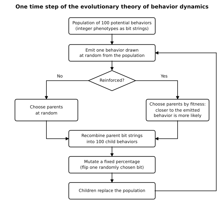
Figure: One time step of McDowell's evolutionary theory of behavior dynamics.

Over many time steps, behaviors in reinforced response classes come to make up more of the population. Because emission is random, the proportion of the population in each class is the probability of emitting that class. Selection by reinforcement changes the population; the population sets the response probabilities.

The ETBD contains no equation for matching and no sensitivity or bias parameter, yet it reproduces the generalized matching law. The artificial organism's response allocation across concurrent schedules converges on matching or near-matching as a result of selection operating on the population of responses. The model also reproduces Herrnstein's hyperbola and patterns of behavioral variability. Its two main parameters are the mean of the fitness density function, which sets how close to the reinforced behavior the selected parents tend to be, and the mutation rate.

Left schedule, RI

30 ticks

Right schedule, RI

60 ticks

FDF mean

40

Mutation rate

10%

RunResetDefault settings

Tick 0 of 30,000. Last 3,000 ticks: proportion of responses from Left = –, of reinforcers = –. Totals: B_L/B_R = –, R_L/R_R = –. Schedule and parameter changes apply from the next tick.

Figure: An artificial organism animated by the ETBD on a concurrent RI 30 RI 60 schedule.

Fitting the generalized matching law to choice data describes the pattern. Showing that a selection process produces matching proposes a mechanism for the pattern. These are different kinds of claims, and both are useful.

Pair 1, Left RI

15 ticks

Pair 1, Right RI

120 ticks

Pair 2, Left RI

20 ticks

Pair 2, Right RI

60 ticks

Pair 3, Left RI

40 ticks

Pair 3, Right RI

40 ticks

Pair 4, Left RI

60 ticks

Pair 4, Right RI

20 ticks

Pair 5, Left RI

120 ticks

Pair 5, Right RI

15 ticks

FDF mean

40

Mutation rate

10%

RunDefault settings

Each pair runs a new organism for 20,000 ticks; the first 5,000 are not counted. R is obtained reinforcers. Press Run to simulate the five schedule pairs.

Figure: The generalized matching law fitted to ETBD artificial organisms, one organism on each of five concurrent RI RI schedules.

Monte Carlo Simulation

Monte Carlo simulation is a family of methods that use repeated random sampling to estimate quantities that are difficult or impossible to compute analytically. You have already used this idea. In Week 8, Otto and Day's stochastic models were analyzed by generating many realizations and summarizing them. Monte Carlo simulation is the general form of that procedure. The method was developed during the Manhattan Project in the 1940s to compute neutron transport through materials, and was named after the Monte Carlo casino.

The logic of Monte Carlo simulations has three steps:

1. Define a model with one or more random components (e.g., probabilistic reinforcement delivery, variable inter-response times, individual differences in learning rate).
2. Run the model many times (hundreds to millions of replications), drawing new random values each time.
3. Analyze the distribution of outcomes across replications.

By the law of large numbers, the average of the simulated outcomes converges on the model's expected value as the number of replications increases. The Monte Carlo error of that average shrinks in proportion to $1/\sqrt{n}$, where $n$ is the number of replications, so any quantity the model defines (a mean, a variance, a probability, an interval) can be estimated to a chosen precision by running more replications.

Uses in behavior science:

• Probabilities of rare events: What is the probability that an organism on a VI 60-s schedule emits 10 responses in 5 seconds? An analytical answer requires the joint distribution of inter-response times and reinforcer set-ups. Simulating the schedule 100,000 times and counting such bursts gives an estimate directly.
• Bootstrap confidence intervals: After fitting a model to data (e.g., sensitivity $a$ and bias $\log b$ in the generalized matching law), resample the data with replacement, refit the model to each resample, and examine the distribution of the estimates. The result is a confidence interval that does not assume the estimate is normally distributed. This matters because estimates from nonlinear models often have skewed sampling distributions, and the Week 8 interval ($\hat{\theta} \pm 1.96 \times SE$) assumes symmetry. In Python, scipy.stats.bootstrap does the resampling.
• Power analysis: Before running an experiment, simulate data under your model with assumed effect sizes and sample sizes, and count how often the planned test detects the effect. This accommodates any model structure and any test statistic, including multilevel models of the kind covered in Week 9.
• Model recovery: Simulate data under each candidate model and ask how often AIC or BIC (Week 6) selects the model that generated the data. This measures whether a given experimental design can distinguish the candidates.
• Sensitivity analysis: Draw parameters from a distribution that reflects uncertainty in their estimates, run the model for each draw, and measure the variance in the output. A large output variance indicates that predictions depend heavily on that parameter.

Monte Carlo simulation is a method, not a model. Any model in this course can be analyzed this way by adding stochastic components and running replications.

Reinforcement Learning (RL)

Reinforcement learning is a computational framework in which an agent learns to select actions by interacting with an environment so as to maximize cumulative reward. The "correct" actions are not explicitly programmed into the agent. Rather, the agent finds out which actions produce the most reward through trial and error. This formalizes the core finding of operant conditioning that behavior changes as a function of its consequences.

An RL problem consists of:

• States ($s$): The situations the agent can be in. In a behavioral experiment, a state might be "left lever extended" or "both levers available after a 5-second changeover delay." In a larger environment, a state might encode location, time since the last reinforcer, the current schedule component, amount of sleep last night, etc.
• Actions ($a$): The behaviors available in each state. For a rat on a concurrent schedule, actions might be "press left lever", "press right lever", or "engage in other behavior". The available actions can differ across states.
• Rewards ($r$): Numerical signals from the environment that follow an action. In behavioral terms, rewards correspond to reinforcers. The agent's objective is to accumulate as much reward as possible over time.
• Policy ($\pi$): A mapping from states to actions. A policy can be deterministic ($\pi(s) = a$) or stochastic ($\pi(a|s)$ gives the probability of each action in each state).
• Value function ($V$ or $Q$): The agent's estimate of the future reward it can expect from a state (or a state-action pair) based on its learning history. The value function is what the agent learns, and the policy is computed from it.

The agent keeps an estimate of the expected future reward for each state or action and updates the estimate after each experience. When an action is followed by more reward than expected, the estimate for that action increases. When it is followed by less, the estimate decreases. The update is driven by prediction error, the difference between expected and obtained reward.

This is the logic of the Rescorla-Wagner model from Week 4: $\Delta V = \alpha \beta (\lambda - V)$, where $(\lambda - V)$ is the prediction error. Reinforcement learning extends it to sequences of decisions in which an action's consequences unfold over time and across states.

RL in AI also distinguishes model-free from model-based learning. A model-free agent, such as a Q-learning agent, learns values directly from experience without representing how the environment works. A model-based agent learns which states lead to which other states, with what probabilities, and uses that representation to choose actions several steps ahead. In behavioral neuroscience the two are often mapped onto habitual responding (model-free) and goal-directed responding (model-based), as measured by sensitivity to outcome devaluation.

Q-Learning

Q-learning is one of the most widely used RL algorithms. It learns a function $Q(s, a)$ that estimates the expected cumulative future reward for taking action $a$ in state $s$ and acting optimally afterward. The "Q" stands for "quality".

The Q-learning update rule is:

$$Q(s, a) \leftarrow Q(s, a) + \alpha \left[ r + \gamma \cdot \max_{a'} Q(s', a') - Q(s, a) \right]$$

Each component:

• $Q(s, a)$: The current estimate of the value of taking action $a$ in state $s$.
• $\alpha$: The learning rate ($0 < \alpha \leq 1$). The fraction of the prediction error added to the estimate on each update.
  • Larger $\alpha$ gives faster learning and larger trial-to-trial fluctuations.
  • Smaller $\alpha$ gives slower learning and smaller fluctuations.
• $r$: The immediate reward received after taking action $a$ in state $s$.
• $\gamma$: The discount factor ($0 \leq \gamma < 1$). The weight given to reward one step in the future relative to immediate reward.
  • When $\gamma = 0$, only immediate reward affects the update.
  • As $\gamma$ approaches 1, future reward is weighted nearly as much as immediate reward.
  • Reward $n$ steps ahead is weighted by $\gamma^n$, which is the exponential discounting function from Week 2 with $\gamma = e^{-k}$ per step.
  • Q-learning therefore discounts at a constant rate per step and, unlike the hyperbolic model, does not predict preference reversals.
• $\max_{a'} Q(s', a')$: The largest Q-value available in the next state $s'$, the agent's current estimate of the best it can do from there.
• $r + \gamma \cdot \max_{a'} Q(s', a') - Q(s, a)$: The temporal difference (TD) error, the difference between what the agent obtained (immediate reward plus the discounted estimate of the future) and what it expected. This is the prediction error that drives learning.

The update moves $Q(s, a)$ toward the obtained reward plus the discounted estimate of the best future. If $\alpha = 1$, the old estimate is replaced by the new information. If $\alpha$ is small (e.g., 0.01), each update is small, and the estimate approximates an average over many experiences.

Q-learning is an off-policy algorithm. It updates toward the value of the best next action (the $\max$), whether or not the agent takes that action next. The agent can therefore learn the values of an optimal policy while still choosing other actions to explore.

The figure below applies the update rule to a rat in a T-maze. On each trial the rat makes three moves: from the start box into the stem, from the stem to the choice point, and from the choice point into one arm. Food is in the arms, so $r = 0$ on the first two moves. Each move updates the Q-value of the move just made. The target looks only one move ahead through $\max_{a'} Q(s', a')$, so the start-box Q-value first rises above 0 on the trial after the stem Q-value does. At asymptote each Q-value is the food value discounted once per move that remains before the food: $r$ for entering the arm, $\gamma r$ at the stem, and $\gamma^2 r$ at the start box. When the rat chooses its arm at random, it enters the empty arm on half the trials, yet the stem Q-value still converges to $\gamma$ times the value of the food arm. This is the off-policy property described above.

$$Q(s,a)\leftarrow Q(s,a)+\alpha \left[r+\gamma \cdot \underset{a^{\prime }}{\max }Q(s^{\prime },a^{\prime })-Q(s,a)\right]$$

Learning rate α

0.30

Discount factor γ

0.90

Food in left arm r

1.0

Food in right arm r

0.0

Arm at the choice point:LeftRightRandom

Next moveFinish trialRun 10 trialsReset

Trial 1. The rat is in the start box, and every Q-value is 0. Dotted lines in B: the values the Q-values converge to when both arms are entered, r in each arm, γ × max r at the stem, and γ² × max r at the start box.

Figure: Q-learning updates for a rat in a T-maze, with the Q-value of each move across trials.

From Rescorla-Wagner to Q-Learning

Placing the two update rules side by side shows the shared structure:

The connection is historical as well as formal. Sutton and Barto, who developed temporal-difference learning in the 1980s, drew on animal learning theory. Barto, Sutton, and Anderson (1983) built a learning system from an "associative search element" and an "adaptive critic element," and described the adaptive critic as a refinement of a model of classical conditioning consistent with Rescorla and Wagner (1972). Sutton (1988) then formalized temporal-difference methods for learning to predict. Schultz, Dayan, and Montague (1997) later reported that the responses of midbrain dopamine neurons in monkeys during conditioning follow a temporal-difference prediction error. Reinforcement learning developed at the intersection of animal learning theory, dynamic programming, and control theory.

Simulation as Experiment

A computational model can be experimented on in ways that are impractical, impossible, or unethical with organisms. For example:

• Parameter sweeps: Vary one parameter across a range while holding the others constant. For instance, sweep $\alpha$ from 0.01 to 1.0 and plot the number of trials to reach steady-state allocation at each value.
• Factorial designs: Cross parameters as you would cross independent variables. Three levels of $\alpha$, three levels of $\gamma$, and four reinforcement-ratio conditions give 36 cells. The output is a simulated data set analyzed with the same tools used for empirical data (ANOVA, regression, multilevel models).
• Many replications: Run thousands of simulated organisms per condition. Monte Carlo error decreases with the number of replications, so the model's predictions can be estimated as precisely as computing time allows. A laboratory experiment might have 6 subjects per condition; a computational experiment can have 10,000.
• Control: Every variable in a simulation is specified by the modeler. There are no equipment failures, illness, or attrition, so differences between conditions are attributable to the manipulated variables and to the random number streams.
• Extreme conditions: Test the model under conditions that cannot be arranged in a laboratory, such as very high reinforcement rates, zero delay, millions of agents, or sessions of millions of trials.
• Counterfactuals: What if the learning rate were zero? What if reinforcement were fully predictable? What if two organisms shared one Q-table?

Results of computational experiments are data about the model, not about organisms. If the model represents the behavior-environment system well, computational experiments generate predictions and suggest empirical studies. If it represents the system poorly, comparisons with data will show that. Keep the two kinds of claims separate: a finding about the model is not a finding about the world until it is tested against data.

---

Applying the 8-Step Framework

We walk through the eight steps for a Q-learning model of concurrent-schedule choice. An agent (an artificial organism) has two response options (two levers) that deliver reinforcement on independent variable-interval (VI) schedules. The question is whether the agent's steady-state allocation follows the generalized matching law, and with what sensitivity.

Step 1: Identify All Environmental and Behavioral Components of the Phenomenon

A rat is placed in an operant chamber with two levers, Left and Right. Left-lever presses are reinforced on a VI 30-s schedule and right-lever presses on a VI 60-s schedule. Once a reinforcer is set up on a lever, it remains available until a press on that lever collects it.

The rat's allocation of responses across the two levers changes with experience of the contingencies. The matching law predicts that at steady state the ratio of left to right responses will equal the ratio of left to right obtained reinforcers, about $2:1$ here. Real concurrent-schedule data usually undermatch, with sensitivity near 0.8 (Week 2).

We want a Q-learning agent that learns an allocation from experience, with no matching rule built in. The model should produce an acquisition period and a steady-state allocation that can be compared with the generalized matching law.

Step 2: Define the Behavioral Principles, Processes, and Intended Scope of the Model

The process of interest is trial-by-trial response allocation on a concurrent VI 30-s VI 60-s schedule. The model includes:

• One agent with no prior history with the contingencies.
• Two actions: press Left, press Right.
• One state: Both levers available. The agent does not distinguish environmental contexts.
• Reinforcement delivery: Determined by two independent VI schedules.
• No changeover delay: The agent can switch between levers on any trial.
• Discrete trials: On each trial, the agent presses one lever and may or may not receive a reinforcer. Each trial represents one second.
• Session length: 3,600 trials, a one-hour session.

Excluded from the model: within-session satiation, fatigue, other behavior (grooming, rearing), the organism's location, response topography, and any pre-existing bias toward one lever.

Step 3: Write Down the Behavioral Principles, Known Quantitative Laws, and Functional Relationships

The governing rule is the Q-learning update:

$$Q(s, a) \leftarrow Q(s, a) + \alpha \left[ r + \gamma \cdot \max_{a'} Q(s', a') - Q(s, a) \right]$$

With a single state, the state notation can be dropped:

$$Q(a) \leftarrow Q(a) + \alpha \left[ r + \gamma \cdot \max_{a'} Q(a') - Q(a) \right]$$

The action-selection rule is a softmax (Boltzmann) policy:

$$P(a_i) = \frac{e^{Q(a_i) / \tau}}{\sum_j e^{Q(a_j) / \tau}}$$

where $\tau$ is a temperature parameter. For two actions, the softmax gives $P(L)/P(R) = e^{[Q(L) - Q(R)]/\tau}$, so the choice ratio depends on the difference between the Q-values divided by $\tau$. As $\tau \to \infty$, choice approaches 50/50 regardless of the Q-values. As $\tau \to 0$, the agent chooses the higher-valued action on every trial.

The scale of $\tau$ must be set relative to the scale of the Q-values. On these schedules a reinforcer follows only a few percent of responses, so the two Q-values differ by a few hundredths. With $\tau = 0.5$ that difference moves $P(L)$ only one or two percentage points from 0.5, and choice stays near 50/50. We use $\tau = 0.1$, the value used in this week's lab.

Temperature τ

0.10

Q(L) − Q(R)

0.033

P(Left) = 0.582. Grey curves: τ = 0.05, 0.1, 0.2, 0.5. Shaded: the steady-state difference in the worked example (±0.033).

Figure: The two-action softmax at four temperatures, with the steady-state Q-value difference from the worked example shaded.

An agent that always chose the higher-valued action would allocate every response to one lever. The softmax produces graded preference, which is required for any allocation between exclusive preference and indifference, including matching.

The reinforcement schedule is modeled as follows. On each trial, time advances by one second. For each lever independently, if no reinforcer is waiting, one is set up with probability $p = 1/\text{VI value}$. Once set up, a reinforcer remains available until the agent presses that lever. A press on a lever with an available reinforcer gives $r = 1$; otherwise $r = 0$.

Step 4: State All Simplifying Assumptions Explicitly

• Single state: The agent does not distinguish moments in the session. It has no representation of time, satiation, or the preceding sequence of responses. Within-session changes in preference come only from the Q-value updates.
• Discrete trials: Concurrent-schedule performance is a free-operant process in continuous time. Discretizing it into one-second trials means the model cannot produce inter-response time distributions or response bursts.
• No changeover delay (COD): Laboratory concurrent schedules usually impose a COD to reduce rapid alternation. Adding one would require at least two states ("just switched" and "stayed").
• Constant parameters: $\alpha$, $\gamma$, and $\tau$ do not change over the session. Organisms' rates of change may decline with experience, and exploration may decrease.
• Independent schedules: The two VI schedules operate independently.
• Stationary environment: The schedule values do not change during the simulation. The model does not address reversals or other contingency shifts.
• Model-free learning: The agent does not learn which actions lead to which states. With one state this has no effect here, but it would matter in a multi-state environment.
• Binary reward: A reinforcer is present ($r = 1$) or absent ($r = 0$). Magnitude, quality, and delay do not vary.

Step 5: Write the Model Verbally, Then Express It Mathematically

Verbally: after each press, the value of the lever just pressed moves a fraction $\alpha$ of the way toward the obtained reinforcer plus the discounted value of the better lever. The next press is chosen with probabilities that increase exponentially with each lever's value.

Next eventFinish trialRun 100 trialsReset

Trial 1, census: Q(L) = 0.000, Q(R) = 0.000.

Figure: The life-cycle diagram for one trial of the Q-learning agent.

Mathematically, the change in the chosen action's value on each trial is:

$$\Delta Q(a) = \alpha \left[ r + \gamma \cdot \max_{a'} Q(a') - Q(a) \right]$$

When $r + \gamma \cdot \max_{a'} Q(a') > Q(a)$, the prediction error is positive and $Q(a)$ increases. When $r + \gamma \cdot \max_{a'} Q(a') < Q(a)$, the prediction error is negative and $Q(a)$ decreases.

Only the chosen action's Q-value is updated on a trial. The value of the other action does not change. The agent obtains information about an alternative only by choosing it, which is why the softmax must allow exploration.

At steady state, the average change in each Q-value is zero. Let $\rho_a$ be the probability that a press on lever $a$ is reinforced. Setting the expected update to zero gives

$$Q^*(a) = \rho_a + \gamma \cdot \max_{a'} Q^*(a')$$

for each lever, and therefore $Q^*(L) - Q^*(R) = \rho_L - \rho_R$. The difference between the two values equals the difference in reinforcers per response. This is the fixed-point concept from Week 10. On a concurrent VI schedule, $\rho_L$ and $\rho_R$ themselves depend on how the agent allocates its responses: pressing a lever more often lowers the probability that any one press on it is reinforced. The fixed point and the allocation must satisfy each other, and with random choice and random set-ups there is no closed-form solution. The model is solved by running it.

This fixed point also shows what Q-learning with a softmax predicts. Strict matching ($B_L/B_R = R_L/R_R$) is the allocation at which reinforcers per response are equal on the two levers, $\rho_L = \rho_R$. At that allocation the two Q-values would be equal, and the softmax would choose each lever equally often, which is not matching. The agent therefore settles between indifference and matching, at an allocation where Left still pays slightly more per response and the Q-value difference sustains a moderate preference. The model predicts undermatching.

Step 6: Verify Dimensional Consistency

• $Q(a)$ is in units of expected cumulative reward (reinforcers, a count).
• $r$ is in the same units as $Q$.
• $\gamma$ is dimensionless ($0 \leq \gamma < 1$).
• $\alpha$ is dimensionless ($0 < \alpha \leq 1$).
• $\gamma \cdot \max_{a'} Q(a')$ is in reward units.
• $r + \gamma \cdot \max_{a'} Q(a') - Q(a)$ is reward units $+$ reward units $-$ reward units, so the prediction error is in reward units.
• $\alpha \cdot [\text{prediction error}]$ is dimensionless $\times$ reward units, so $\Delta Q(a)$ is in reward units.
• $\tau$ is in reward units, so $Q(a)/\tau$ in the softmax exponent is dimensionless, as an exponent must be.

Units check.

Step 7: Specify Starting Values and Constraints

• Initial Q-values: $Q(\text{Left}) = 0$, $Q(\text{Right}) = 0$. The agent has no history with either lever. Equal starting values make the softmax give each lever probability 0.5 on the first trial.
• Constraints: Q-values can take any real value. With a minimum reward of zero and nonnegative starting values, they remain nonnegative. They grow toward roughly $\rho/(1 - \gamma)$, where $\rho$ is the probability that a press is reinforced, so with $\gamma = 0.95$ they settle near 1 rather than near the per-press reinforcement probability.
• Simulation length: 3,600 trials. Steady state is assessed over the second half of the session (trials 1,801–3,600).

Step 8: Check the Math, Test Against Data, and Derive Predictions

Verification (does the program do what we specified?):

• Hand-trace the first several updates and compare with the program's output (see the Worked Example below).
• Check that the softmax returns probabilities consistent with the Q-values and $\tau$.
• Check the VI logic: reinforcers should be set up at the programmed average rates and collected only by a press on the correct lever.
• Check boundary behavior: equal Q-values should give equal choice probabilities; a Q-value difference much larger than $\tau$ should give nearly exclusive choice.

Validation (does the model reproduce empirical regularities?):

• Run the simulation many times and compute the steady-state allocation in each run.
• Compare the response ratio $B_L / B_R$ with the obtained reinforcer ratio $R_L / R_R$.
• Run several reinforcement ratios (e.g., VI 20-s VI 60-s, VI 30-s VI 30-s, VI 60-s VI 20-s), fit the generalized matching law to the steady-state ratios, and compare the fitted sensitivity $a$ and bias $\log b$ with values from concurrent-schedule experiments.

Solving the model means running it. The logistic ODE from Week 10 has a closed-form solution. This model's fixed point is defined by the equation in Step 5, but the allocation that satisfies it has to be found by simulation. The output is a time series of choices, reinforcers, and Q-values that we analyze numerically.

---

Worked Example

We implement a Q-learning agent choosing between two levers on a concurrent VI 30-s VI 60-s schedule with these values:

• Learning rate: $\alpha = 0.1$
• Discount factor: $\gamma = 0.95$
• Temperature: $\tau = 0.1$
• Initial Q-values: $Q(\text{Left}) = 0$, $Q(\text{Right}) = 0$
• Trial duration: 1 second
• Set-up probabilities per trial: $p_L = 1/30 \approx 0.0333$, $p_R = 1/60 \approx 0.0167$
• Number of trials: 3,600 (one hour)

Schedule Mechanics

On each trial, for each lever independently, a reinforcer is set up with probability $p$ if none is already waiting on that lever. Once set up, it stays available until collected. A press on a lever with an available reinforcer gives $r = 1$ and removes the reinforcer.

This implements the property of VI schedules that matters for choice: reinforcers continue to be set up on one lever while the agent presses the other. If the agent presses Left for many consecutive trials, a reinforcer is likely to be waiting on Right when it next switches. Responding exclusively to one lever leaves reinforcers uncollected on the other, so allocations between the two levers obtain more reinforcers than exclusive preference does.

Simulation Trace: First Five Trials

The first five trials below use a fixed sequence of choices and outcomes so the arithmetic can be followed. In a real run each outcome is random.

Trial 1: $Q(L) = 0$, $Q(R) = 0$. The softmax gives $P(L) = P(R) = 0.5$. The agent presses Left, and a reinforcer is waiting ($r = 1$).

$$Q(L) \leftarrow 0 + 0.1 \times [1 + 0.95 \times \max(0, 0) - 0] = 0 + 0.1 \times 1.0 = 0.100$$

The prediction error is $1.0$: the agent expected nothing and received a reinforcer.

Trial 2: $Q(L) = 0.100$, $Q(R) = 0$. The softmax gives $P(L) = \frac{e^{0.100/0.1}}{e^{0.100/0.1} + e^{0/0.1}} = \frac{e^{1}}{e^{1} + 1} = \frac{2.718}{3.718} \approx 0.731$. A difference of 0.1 between the Q-values, equal to $\tau$, already produces a clear preference. The agent presses Left, and no reinforcer is waiting ($r = 0$).

$$Q(L) \leftarrow 0.100 + 0.1 \times [0 + 0.95 \times 0.100 - 0.100] = 0.100 + 0.1 \times (-0.005) = 0.0995$$

The prediction error is $0.095 - 0.100 = -0.005$. With no reinforcer, the target is only the discounted value of the best lever, which is slightly less than the current estimate, so $Q(L)$ decreases slightly.

Trial 3: $Q(L) = 0.0995$, $Q(R) = 0$. $P(L) \approx 0.730$. The agent presses Right (the less probable choice), and a reinforcer is waiting ($r = 1$).

$$Q(R) \leftarrow 0 + 0.1 \times [1 + 0.95 \times \max(0.0995, 0) - 0] = 0.1 \times 1.0945 = 0.1095$$

The target includes the discounted value of Left ($0.95 \times 0.0995 = 0.0945$), because the $\max$ is taken over both actions in the single state. This is bootstrapping: the value of Right is updated partly from the current estimate of Left.

Trial 4: $Q(L) = 0.0995$, $Q(R) = 0.1095$. $P(L) \approx 0.475$. The agent presses Right, and no reinforcer is waiting ($r = 0$).

$$Q(R) \leftarrow 0.1095 + 0.1 \times [0 + 0.95 \times 0.1095 - 0.1095] = 0.1095 + 0.1 \times (-0.0055) = 0.1089$$

Trial 5: $Q(L) = 0.0995$, $Q(R) = 0.1089$. $P(L) \approx 0.477$. The agent presses Left, and a reinforcer is waiting ($r = 1$).

$$Q(L) \leftarrow 0.0995 + 0.1 \times [1 + 0.95 \times 0.1089 - 0.0995] = 0.0995 + 0.1 \times 1.0040 = 0.1999$$

After five trials, $Q(L) = 0.200$ and $Q(R) = 0.109$. The gap reflects which presses happened to be reinforced in this short sequence, not the 2:1 programmed ratio. Over a session, each Q-value tracks the probability that a press on that lever is reinforced, plus the discounted value of the better lever.

Q-Values and Allocation Across the Session

The figure below summarizes 500 independent runs of the full simulation. Panel A shows the mean Q-value of each lever across trials. Panel B shows the mean proportion of left presses in 100-trial bins, with the middle half of runs shaded.

Learning rate α

0.10

Discount factor γ

0.95

Temperature τ

0.10

Left schedule, VI

30 s

Right schedule, VI

60 s

Chapter valuesNew random runs

500 runs of 3,600 trials. Second half: P(Left) = 0.568 (B_L/B_R = 1.31); proportion of reinforcers from Left = 0.667 (R_L/R_R = 2.01). Shaded: middle half of runs.

Figure: Q-values and choice across a one-hour session, averaged over 500 runs.

Over the second half of the session (trials 1,801–3,600), the agent made 56.7% of its presses on Left (SD across runs 0.026) and obtained 66.6% of its reinforcers there. Strict matching would place 66.7% of presses on Left.

Interpreting the Results

1. Both Q-values rise toward the same level: Both values increase over the session because $\gamma = 0.95$ adds the discounted value of the better lever to every update. By the end of the session they differ by about 0.03. The difference, not the level, determines choice, and it is consistent with the Step 5 result that $Q^*(L) - Q^*(R) = \rho_L - \rho_R$.

2. Preference develops early and then partly reverses: Preference for Left peaks at about 0.63 within the first 300 trials and then declines to about 0.57. Early in the session the Q-values are small and the more frequently chosen lever's value is inflated by the $\gamma \max Q$ term. As both values approach their steady-state level, the difference between them shrinks toward the difference in reinforcers per response.

3. Allocation undermatches: The steady-state response ratio is $B_L/B_R = 1.32$ (mean across runs) against an obtained reinforcer ratio of $R_L/R_R = 2.07$. Behavior is distributed more evenly than reinforcement, as Step 5 predicted.

4. The agent was not given a matching rule: No matching equation appears in the model. The allocation is a result of prediction-error updates, the softmax, and the VI contingencies. What the model produces is undermatching, a result that can be compared with data, not an assumption.

5. The allocation depends on $\tau$: With $\tau = 0.2$, steady-state $P(\text{Left})$ falls to about 0.54. With $\tau = 0.5$, it is about 0.51. Smaller values of $\tau$ move allocation toward matching but increase the chance that the agent locks onto one lever early in the session and does not sample the other again. Sensitivity to reinforcement in this model is set largely by $\tau$ relative to the scale of the Q-values.

Running Multiple Replications

A single run is one realization of a stochastic process. Each run involves random set-ups and random choices, and a different random seed gives a different trajectory.

To estimate what the model predicts, we ran the simulation 500 times with the same parameters and different seeds. Across replications, the steady-state ratio $B_L / B_R$ had a mean of 1.32 and an SD of 0.21. The middle 95% of replications fell between 1.10 and 1.59, and the 95% confidence interval for the mean was $[1.31, 1.34]$. The SD describes how much one simulated organism varies; the confidence interval describes how precisely 500 replications estimate the model's average.

To estimate sensitivity, we repeated the procedure for five schedule pairs (VI 20-s VI 60-s, VI 30-s VI 60-s, VI 30-s VI 30-s, VI 60-s VI 30-s, VI 60-s VI 20-s), fit the generalized matching law to the five log ratios, and replicated the whole procedure 100 times. The median fitted sensitivity was $a = 0.44$, and 2.5% of replications fell below 0.38. A few replications gave estimates above 1 (the largest was 1.46), so the distribution has a long right tail and the median is the better summary. Bias was near zero (mean $\log b = -0.005$, SD 0.03, base-10 logs), as expected for an agent that treats the two levers identically.

Learning rate α

0.10

Discount factor γ

0.95

Temperature τ

0.10

Chapter valuesNew random runs

Five schedule pairs (VI 20/60, 30/60, 30/30, 60/30, 60/20), 3,600 trials each, second half. Median a = 0.44; mean log b = 0.000. Panel A shows the replication closest to the median (a = 0.44).

Figure: The generalized matching law fitted to the agent's steady-state allocation across five schedule pairs.

With these parameters, Q-learning undermatches, with sensitivity well below the value of about 0.8 typical of pigeon data (Week 2). This week's lab repeats this analysis and adds a bootstrap interval on the steady-state allocation.

This is Monte Carlo simulation applied to a model: many replications of a stochastic process, summarized with the same statistics used for empirical data.

---

Plain-Language Interpretation

What Q-Learning Says in Everyday Terms

Q-learning keeps a number for each action. After each action, it compares what happened with what it expected. If the outcome was better than expected, the number for that action goes up. If it was worse, the number goes down. Over time the numbers settle near the long-run reinforcement each action produces, and the agent chooses higher-numbered actions more often.

A rat responding on two levers does not solve the matching equation. It responds, contacts consequences, and its allocation changes. Responses followed by reinforcement occur more often; responses not followed by reinforcement occur less often. Q-learning states one version of this process as an algorithm in which the size of each change depends on the difference between the expected and obtained outcome.

Q-learning is "model-free" in the same sense. The agent does not learn that the left lever sets up food on average every 30 seconds. It learns that the left lever's value is 1.27 and the right lever's value is 1.24. This is close to the behavior-analytic emphasis on functional relations between behavior and its consequences.

What Emergence Means

When we say an allocation "emerges" from Q-learning, we mean that no allocation rule was written into the model. The allocation results from the learning algorithm interacting with the reinforcement contingencies. Patterns at the molar level can result from rules at the molecular level without being specified by the modeler.

Emergence gives a different kind of account from curve fitting. Fitting the generalized matching law to data describes the pattern. Showing that a learning mechanism produces a particular allocation is a process account as it proposes how the pattern arises. The process account can also be wrong in testable ways. This week's model, for example, predicts undermatching whose degree depends on the softmax temperature, and that prediction can be compared with data.

---

Assumptions and Limitations

Discrete States and Actions

Tabular Q-learning assumes that states and actions are discrete and finite, and it stores one value per state-action pair. Behavior also varies along continuous dimensions. For example, a lever press varies in force, speed, and duration; and an organism's location varies continuously. A table cannot represent this, and a problem with millions of states would need millions of entries, each visited many times. Deep reinforcement learning, including deep Q-networks (DQN), replaces the table with a neural network that generalizes from visited states to similar unvisited ones. The cost is additional complexity and less stable learning.

Stationary Environment Assumption

Standard Q-learning assumes that the reward structure does not change. When schedules shift within a session (reversals, multiple schedules, progressive-ratio schedules), the Q-values lag behind the new contingencies by a number of trials that depends on $\alpha$. Higher learning rates, eligibility traces, and other modifications reduce the lag. Cox (2026, preprint; a Week 10 supplemental reading) compares reinforcement learning models with behavior-dynamic and behavioral-ecology models in a two-choice task whose reinforcement rates change within a session, evaluating them on the path of allocation over time rather than on its endpoint.

Model-Free Limitation

A model-free agent learns only from direct experience. It cannot evaluate the consequences of a sequence of actions before taking it. Model-based algorithms learn transition probabilities and reward functions and use them to evaluate actions in advance, which lets them learn from fewer experiences. The costs are more computation and errors when the learned representation is inaccurate.

Cost and Interpretability

Large computational models require substantial computing time, which limits how many conditions can be run. They can also be difficult to interpret. For example, a large ABM may predict accurately while the reason for its predictions remains unclear. These are the limitations described at the start of the chapter and the primary reason that computational models are used alongside analytical ones.

---

Connection to Empirical Behavior Science

McDowell's Evolutionary Theory of Behavior Dynamics

McDowell (2019) reviews the current status of the ETBD, in which behavior is treated as a population of potential behaviors undergoing selection by reinforcement, recombination, and mutation. Artificial organisms animated by the theory reproduce the generalized matching law, Herrnstein's hyperbola, and patterns of behavioral variability without those relations being written into the model. The theory has been tested against data from concurrent schedules, single-alternative schedules, and other procedures, and McDowell discusses where the artificial organisms' behavior agrees and disagrees with that of live organisms.

Cox and Santos (2025) on AI-Based RL and Behavior Science

Cox and Santos (2025) describe how reinforcement learning in artificial intelligence differs from operant research and how each field can inform the other. To demonstrate, they built 12 artificial organisms to predict the next response emitted by each of six human participants. Each artificial organism used one of six combinations of feature sets informed by operant research, with or without punishment of incorrect predictions. A thirteenth approach used Q-learning to update context-response-outcome values after each response and to choose the next response. That approach had the highest mean predictive accuracy (95%, range 90%–99%).

Matching as a Result of Learning Processes

Three mechanisms in this course now produce steady-state allocation that relates to relative reinforcement without a matching rule written in. The competition model in Week 10 places a stable equilibrium on a matching relation, with sensitivity $(1+a)/(1-a) \geq 1$, so it produces strict matching or overmatching. McDowell's ETBD produces matching or near-matching. Q-learning with a softmax, as shown above, produces undermatching whose degree depends on $\tau$. The matching law may therefore be a consequence of more basic reinforcement processes rather than a principle in its own right. Which mechanism, if any, is correct is an empirical question.

If matching results from a learning process, then deviations from matching (undermatching, overmatching, bias) may reflect properties of that process, such as learning rate and exploration, rather than free parameters of a descriptive equation. Week 10 noted that the competition model cannot produce undermatching without an added term. Q-learning produces it from exploration alone. Computational models can test such hypotheses by varying the learning parameters and comparing the resulting deviations with data.

Agent-Based Models of Social Behavior

ABMs have also been applied to social behavior such as cooperation, cultural transmission, norm formation, and group decision-making. Agents with behavioral rules interact in structured environments, and the models examine how individual reinforcement histories produce group-level patterns. This question is difficult to address with equation-based models alone. For example, an ABM of cooperation can show reciprocal cooperation arising among agents that each follow a tit-for-tat rule.

---

Connecting Forward: From Implementing Rules to Discovering Them

Every model this week started from a specified mechanism. We told the Q-learning agent how to update its values and choose. McDowell specified how selection, recombination, and mutation work. An ABM's modeler specifies each agent's rules. Running the model shows what those mechanisms produce, but the mechanisms come from the modeler and from behavioral theory.

Next week reverses the direction. Machine learning starts with data and searches for a function that maps inputs to outputs, without the modeler specifying the process that generated the data. This week's models ask "What does this mechanism produce?" ML asks "What function best predicts these data?" The prediction-error update used this week is also the basis of the gradient-based training used in much of modern ML. The goals differ across the two. Computational models in behavior science are usually built to explain, and ML models are usually built to predict. Week 12 covers when prediction without explanation is useful, when it is not, and how the two approaches can be combined.

---

Exercises for Reflection

1. In the worked example, the Q-learning agent undermatched on a concurrent VI 30-s VI 60-s schedule with $\gamma = 0.95$. What would happen if you changed the discount factor to $\gamma = 0$? Use the fixed-point equation from Step 5 to predict how the Q-values and the allocation would change, and explain your reasoning in terms of what $\gamma$ does to the prediction error.

2. The Week 10 competition model produces matching or overmatching, McDowell's evolutionary model produces matching or near-matching, and Q-learning with a softmax produces undermatching. What does this tell us about the status of the matching law as a scientific principle? What data would distinguish among the three mechanisms? Can you think of other examples in science where the same regularity arises from several distinct mechanisms?

3. A colleague argues that computational models are "curve fitting with extra steps": they have so many parts that they can fit any data. How would you respond? What distinguishes a computational model that explains from one that reproduces the data it was built to fit? Consider the roles of a priori predictions, number of free parameters, and emergent properties in your answer.

4. You want to build an agent-based model of a classroom in which students' on-task behavior is influenced by teacher-delivered reinforcement and peer attention. What would be the agents, states, rules, and environment? What group-level patterns might emerge, and how would you test whether the model produces realistic dynamics?

---

Key Readings

McDowell (2019) reviewed the current status of the evolutionary theory of behavior dynamics (ETBD), a computational model that treats operant behavior as a population of potential behaviors that undergoes selection by reinforcement, recombination of parent behaviors, and mutation on each time step. Unlike the closed-form models from earlier weeks (matching, discounting, demand), the ETBD derives molar regularities, including matching and Herrnstein's hyperbola, from rules implemented as an algorithm that must be run rather than solved. The paper shows the defining feature of computational models: behavioral patterns result from simple rules iterated over time, and what those rules predict is found by simulating them.

Cox and Santos (2025) compared operant research and AI-based reinforcement learning and demonstrated how combining them can improve prediction of individual responses. For six human participants, they built artificial organisms using different combinations of operant-informed feature sets, with and without punishment of incorrect predictions, and a separate Q-learning approach that updated context-response-outcome values after each response. The Q-learning approach predicted the next response most accurately (mean 95%). The RL framework descends from the prediction-error idea of the Rescorla-Wagner model (Week 4), and the paper connects that earlier material to current AI methods. It also raises the question of whether RL models could support real-time decisions in applied behavior analysis.

---

Reading Guide

McDowell (2019)

• What is the evolutionary theory of behavior dynamics (ETBD), and how does it differ from traditional mathematical models of behavior?
• How does the ETBD use concepts from evolutionary biology (selection, variation, reproduction) to model operant behavior?
• What is the "population of behaviors" concept in the ETBD? How does this differ from treating behavior as a single response rate?
• How does reinforcement operate in the ETBD? What is being "selected"?
• What predictions does the ETBD make about matching, and how do these compare to the predictions of Herrnstein's hyperbola?
• Does the ETBD derive matching from first principles, or is matching built into its assumptions? Why does this distinction matter?
• What role does mutation play in the ETBD? How does it relate to behavioral variability?
• How does the ETBD handle phenomena like extinction and spontaneous recovery?
• What is the relationship between the ETBD and the generalized matching law? Does the ETBD predict sensitivity and bias parameters?
• What empirical evidence does McDowell cite in support of the ETBD?
• What are the main criticisms or limitations of the ETBD that McDowell acknowledges?
• How does the ETBD relate to other computational approaches to behavior (e.g., reinforcement learning, neural networks)?
• Why does McDowell argue that computational models like the ETBD are valuable even when closed-form equations exist?
• What does it mean to say the ETBD is a "generative" model? How does this differ from a descriptive or curve-fitting model?
• What are the implications of the ETBD for understanding behavior at a mechanistic level?

Cox & Santos (2025)

• What is the central argument of the paper regarding the integration of AI-based reinforcement learning (RL) with behavior science?
• How do the authors define reinforcement learning in the AI/computational sense? How does this relate to the behavioral definition of reinforcement?
• What specific RL algorithm is used in the paper, and how does it work?
• What behavioral preparation or task do the authors model using RL?
• What does "predicting the next response" mean in this context? How is it different from predicting aggregate response rates?
• How well does the RL model perform at predicting individual responses? What metrics are used to evaluate performance?
• What are the parallels between Q-learning parameters (learning rate, discount factor) and behavioral concepts?
• How do the authors address the concern that computational models are "black boxes" that don't explain behavior?
• What implications does this work have for applied behavior analysis? Could RL models inform treatment decisions?
• How does this paper connect to the matching law and other quantitative models covered earlier in the course?
• What are the limitations of the approach, as discussed by the authors?
• What does this paper suggest about the future relationship between AI/ML and behavior science?
• How does this work differ from McDowell's ETBD in its approach to computational modeling of behavior?
• Why is predicting individual responses (molecular level) important in addition to predicting molar measures like response rates?

---

References

Barto, A. G., Sutton, R. S., & Anderson, C. W. (1983). Neuronlike adaptive elements that can solve difficult learning control problems. IEEE Transactions on Systems, Man, and Cybernetics, SMC-13(5), 834--846. https://doi.org/10.1109/TSMC.1983.6313077

Cox, D. J. (2026). Testing behavior dynamic models to predict choice in a non-stationary two-choice foraging environment [Preprint].

Cox, D. J., & Santos, C. (2025). Predicting the next response: Demonstrating the utility of integrating artificial intelligence-based reinforcement learning with behavior science. Perspectives on Behavior Science, 48, 241--267. https://doi.org/10.1007/s40614-025-00444-6

McDowell, J. J. (2019). On the current status of the evolutionary theory of behavior dynamics. Journal of the Experimental Analysis of Behavior, 111(1), 130--145. https://doi.org/10.1002/jeab.495

Rescorla, R. A., & Wagner, A. R. (1972). A theory of Pavlovian conditioning: Variations in the effectiveness of reinforcement and nonreinforcement. In A. H. Black & W. F. Prokasy (Eds.), Classical conditioning II: Current research and theory (pp. 64--99). Appleton-Century-Crofts.

Schultz, W., Dayan, P., & Montague, P. R. (1997). A neural substrate of prediction and reward. Science, 275(5306), 1593--1599. https://doi.org/10.1126/science.275.5306.1593

Sutton, R. S. (1988). Learning to predict by the methods of temporal differences. Machine Learning, 3(1), 9--44. https://doi.org/10.1007/BF00115009

---

Key Takeaways

• Computational models implement behavioral processes as algorithms that are run rather than solved; the model is the program.
• Agent-based models (ABMs) specify rules for individual agents, and group-level patterns result from their interactions. McDowell's evolutionary theory of behavior dynamics emits behaviors at random from a population and changes the population by reinforcement-driven parent selection, recombination, and mutation; it reproduces the matching law without a matching rule.
• Monte Carlo simulation uses repeated random sampling to estimate probabilities, distributions, and intervals for model outputs. It extends the simulation approach from Week 8 and is a method, not a model family.
• Reinforcement learning (RL) is a computational framework in which an agent learns to maximize cumulative reward through trial-and-error interaction with an environment. It formalizes the operant finding that behavior changes as a function of its consequences.
• Q-learning updates state-action values using $Q(s,a) \leftarrow Q(s,a) + \alpha[r + \gamma \cdot \max_{a'} Q(s',a') - Q(s,a)]$, driven by the temporal-difference prediction error. The discount factor $\gamma$ is exponential discounting (Week 2).
• Rescorla-Wagner and Q-learning both change an estimate by a fraction of a prediction error. Q-learning adds states, actions, temporal discounting, and bootstrapping, and reduces to a Rescorla-Wagner form when $\gamma = 0$ with a single state.
• At steady state, the difference between two Q-values equals the difference in reinforcers per response. Because strict matching equalizes reinforcers per response, a Q-learning agent with a softmax policy undermatches, and its sensitivity depends on the temperature $\tau$.
• Q-learning is model-free: the agent learns from contact with outcomes without representing the environment's structure.
• Computational models can be experimented on: parameters can be swept, factorial designs run, and thousands of replications generated with full control over every variable.
• Limitations include discrete states and actions, the stationarity assumption, model-free learning, computational cost, and lower interpretability than analytical models.
• The 8-step framework applies to computational models: identify the components, define the scope, write the update and choice rules, state assumptions, express the model verbally and mathematically, check units, specify starting values, and verify and validate by running the simulation.
• Prediction error links behavior science and AI: from Rescorla-Wagner, through temporal-difference learning, to current reinforcement learning. The dopamine prediction-error findings are evidence that neural systems compute a similar signal.